Using SUMIF to Add Values Within a Date Range

While working in Excel, we often need to sum values from a table based on a certain condition. In this tutorial, we will learn how to sum values with specific conditions using the SUMIFS function.

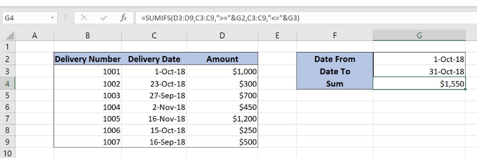
Figure 1. Final result

Syntax of the SUMIFS formula

=SUMIFS(sum_range, criteria_range1, criteria1, criteria_range2, criteria2)

The parameters of the SUMIFS function are:

• sum_range – a range with values which we want to sum
• criteria_range1 – a range where we want to set our first condition
• criteria1 – the first condition for summing the values
• criteria_range2 – a range where we want to set our second condition
• criteria2 – the second condition for summing the values

Setting up Our Data for the SUMIFS Function

Our table consists of 3 columns: “Delivery Number” (column B), “Delivery Date” (column C) and “Amount” (column D). In cells G2 and G3, we specify a date range, while in cell G4 we want to get a sum between dates.

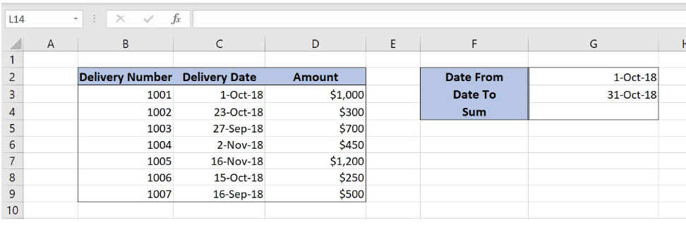Figure 2. Data that we will use in the SUMIFS example

Sum Amount Between Two Value Ranges Using the SUMIFS Function

In our example, we want to sum all amounts from column D that are between 1-Oct-18 and 31-Oct-18.

Formula:

=SUMIFS(D3:D9, C3:C9, ">="&G2, C3:C9, "<="&G3)

The sum_range is D3:D9. Criteria1 is “>=”&G2. As our first criteria is the date greater than or equal to G2 (1-Oct-18). Criteria2 is “<=”&G3

To apply the SUMIFS function, we need to follow these steps:

• Select cell G4 and click on it
• Insert the formula: =SUMIFS(D3:D9, C3:C9, ">="&G2, C3:C9, "<="&G3)
• Press enter

Figure 3. Using the SUMIFS function to sum values between two dates

In this example, we get all amounts which have the corresponding date between 1-Oct-18 and 31-Oct-18. As you can see, rows 3 (1-Oct-18), 4 (23-Oct-18) and 8 (15-Oct-18) meet both conditions, so correspondings amounts are summed ($1,000, $300, $250). Finally, the sum in the cell G4 is $1,550.

Most of the time, the problem you will need to solve will be more complex than a simple application of a formula or function. If you want to save hours of research and frustration, try our live Excelchat service! Our Excel Experts are available 24/7 to answer any Excel question you may have. We guarantee a connection within 30 seconds and a customized solution within 20 minutes.