

We sum the values using the SUMIF function where cell value is equal to the criteria value. However, we can also sum the values where cell isn’t equal to the criteria value. This step by step tutorial will help all levels of Excel users learn how to use the SUMIF function to sum all values that aren’t equal to the criteria value
SUMIF Function
=SUMIF(range, “<>criteria”, [sum_range])
Where comparison operator “not equal to” needs to enclose in double quotation marks (“ “). The SUMIF function sums the value if the value in the corresponding range is not equal to criteria value.
SUMIF a Cell is Not Blank
If we want to sum the value of a cell that is not blank or empty, then the SUMIF is very handy to deal with such value. We only need to use comparison operator “Not equal to” (<>) in the criteria argument and the SUMIF function sums up all the cells in the sum_range argument that are not empty or blank. Suppose we want to sum the amounts in range C2: C11 where the delivery date in range D2: D11 is not blank or empty. The SUMIF formula will be as follows:
=SUMIF(D2:D11,"<>",C2:C11)
![]() Figure 1. SUMIF a Cell is Not Blank
Figure 1. SUMIF a Cell is Not Blank
SUMIF a Cell is Not Equal to Exact Match
When we want to exclude the value to sum that is equal to an exact match of criteria value, then the operator “Not equal to” (<>) is used with criteria value in criteria argument of the SUMIF function. Suppose we do not want to sum the orders’ amounts of “Biscuits” in total, the SUMIF function will exclude the amounts of orders that belong to the product “Biscuits” in range B2: B11, while summing up the amounts in range C2: C11.
=SUMIF(B2:B11,"<>Biscuits",C2:C11)
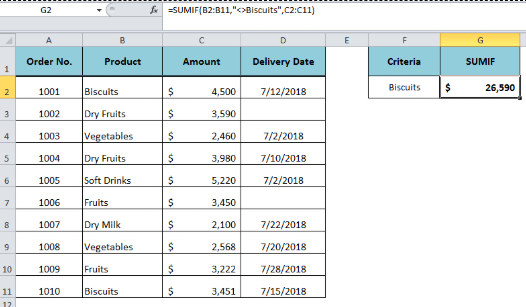 Figure 2. SUMIF a Cell is Not Equal to Exact Match
SUMIF a Cell is Not Equal to Partial Match
The SUMIF function supports wildcard characters, such as the asterisk (*) and the question mark symbol (?), to sum the values based on the partial match to the criteria value. But if we want to sum a value if the corresponding cell does not contain the criteria value in any combination, with or without any other word, then this can be done using the operator “Not equal to” along with the asterisk wildcard in criteria argument of the SUMIF function. Suppose we do not want to sum the orders’ amounts in range C2: C11 where the corresponding cell in the range B2: B11 contains the word “Fruits” in any combination.
=SUMIF(B2:B11,"<>*Fruits*",C2:C11)
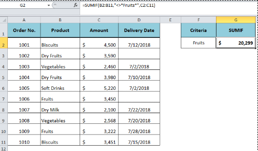 Figure 3. SUMIF a Cell is Not Equal to Partial Match
SUMIF a Cell is Not Equal to Criteria with Cell Reference
We can use cell reference to replace the criteria value in the SUMIF function. Similarly, we can sum a value that is not equal to criteria with a cell reference. Suppose we have our criteria value in a cell reference and we want to use this cell reference instead of a direct value in criteria. In this case, we will concatenate the cell reference with the operator “Not equal to” (<>) in criteria argument using the ampersand (&). Suppose we want to sum the amounts in range C2: C11 where the corresponding cell in the range B2: B11 is not equal to value “Fruits” given in cell reference F2. The SUMIF formula would be as follows;
=SUMIF(B2:B11,"<>"&F2,C2:C11)
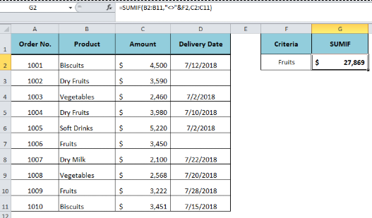 Figure 4. SUMIF a Cell is Not Equal to Criteria with Cell Reference
Instant Connection to an Expert through our Excelchat Service:
Most of the time, the problem you will need to solve will be more complex than a simple application of a formula or function. If you want to save hours of research and frustration, try our live Excelchat service! Our Excel Experts are available 24/7 to answer any Excel question you may have. We guarantee a connection within 30 seconds and a customized solution within 20 minutes.


Leave a Comment