

There are several functions in Excel that are useful in finding a given value in a range of cells, such as the SUMIF, INDEX and MATCH functions. This step by step tutorial will assist all levels of Excel users in comparing the lookup functions of SUMIF, INDEX and MATCH.
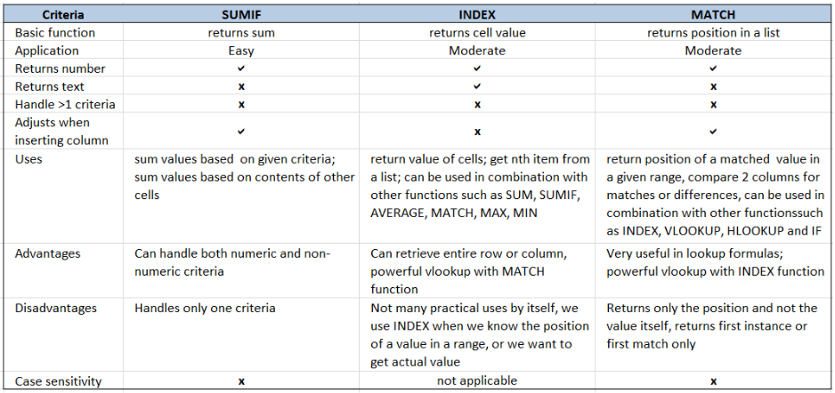 Figure 1. Final result: Comparison of SUMIF, INDEX and MATCH
Syntax of the SUMIF Function
SUMIF sums the values in a specified range, based on one given criteria
=SUMIF(range,criteria, [sum_range])
- Range: the data range that will be evaluated using the criteria
- Criteria: the criteria or condition that determines which cells will be added
- Sum_range: the cells that will be added; if left blank, “sum_range” = “range” which means that the range of data that will be added is the same range of data evaluated
Syntax of the INDEX function
INDEX function returns a value from within a range, as specified by the row and column number
=INDEX(array, row_num, column_num)
- array – a range of cells where we want to retrieve some data
- row_num – the row in the array from which we want to retrieve data
- column_num – the column in the array from which we want to retrieve data; if the array has only one column, column_num can be omitted
Syntax of the MATCH function
MATCH function returns the position of a value in a range
=MATCH(lookup_value, lookup_array, [match_type])
- lookup_value – a value which we want to find in the lookup_array
- lookup_array – the range of cells containing the value we want to match
- [match_type] – optional; the type of match; if omitted, the default value is 1; We use 0 to find an exact match
Setting up Our Data
Our table consists of two columns: Product (column B) and Orders (column C). We will use this data to show some of the uses of SUMIF, INDEX and MATCH functions.
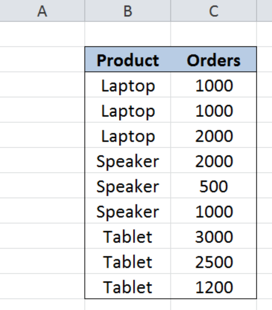 Figure 2. Sample data for comparison of SUMIF, INDEX and MATCH
SUMIF
The SUMIF function sums the values in a specified range based on one given criteria. In the table below, SUMIF is used to add values that satisfy three different criteria.
- Sum of orders that are equal to 1000
- Sum of orders for “Laptop”
- Sum of orders for orders greater than 2000
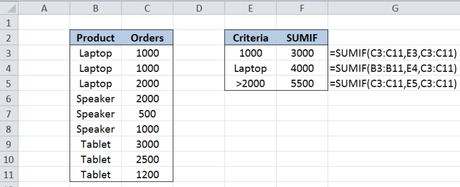 Figure 3. Actual uses of SUMIF function
SUMIF is very easy to use, and its syntax is straightforward. We determine the range of data to be evaluated, the criteria, and the range to be added.
We use SUMIF when we want to calculate the sum of values based on its contents, or the contents of other cells. However, SUMIF can only handle one given criteria. For multiple criteria, we can use the SUMIFS instead of SUMIF.
INDEX
INDEX function returns a value from within a range, as specified by the row and column number. We use INDEX when we know the position of the value in a range or when we want to get the nth item in the list. INDEX can also be used to retrieve the values in an entire row or column.
When used by itself, the INDEX function has very few uses, but when combined with other functions, INDEX becomes one of the most powerful functions in Excel.
In the table below, INDEX is used to :
- Get the value of the cell in the 2nd row, 2nd column
- Sum all orders in column C; in combination with SUM function
- Sum orders greater than 2000; in combination with SUMIF function
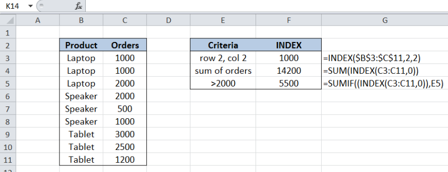 Figure 4. Actual uses of INDEX function
INDEX is easy to use for its basic purpose of returning the value of a cell. However, it takes practice and a little mastery when we use INDEX in combination with other functions especially in looking up values.
MATCH
MATCH function returns the position of a value in a range. We use MATCH when we want to determine the position only, and not the actual value itself. Just like INDEX, the MATCH function also has few uses when used by itself. However, using it with other functions, especially with INDEX, it can create a powerful lookup formula.
In the table below, MATCH is used to :
- Get the position of the first match of Tablet in the list
- Get the position of the first 2000 orders in the list
- Get the position of the first 2500 orders in the list
- Determine if a value is present in a list; in combination with the IF and ISNA functions
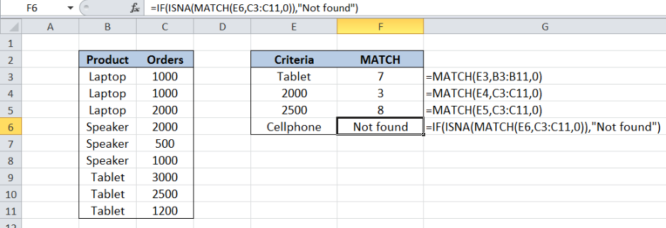 Figure 5. Actual uses of MATCH function
Comparison of SUMIF, INDEX, MATCH
Below table summarizes the uses, advantages and disadvantages of the SUMIF, INDEX and MATCH functions.
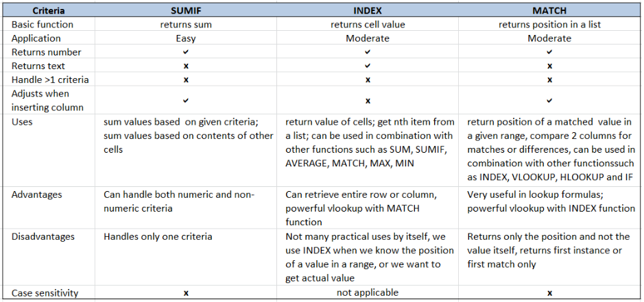 Figure 6. Comparison of SUMIF, INDEX, MATCH
Comparison of the three functions shows merits for each of them, and each has its own advantages and disadvantages. The value of each function is only as good as how a user uses them in a formula.
Most of the time, the problem you will need to solve will be more complex than a simple application of a formula or function. If you want to save hours of research and frustration, try our live Excelchat service! Our Excel Experts are available 24/7 to answer any Excel question you may have. We guarantee a connection within 30 seconds and a customized solution within 20 minutes.


Leave a Comment