

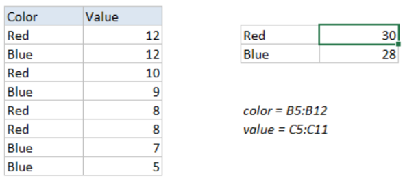
 Figure 1. of Sum Top Values with Criteria.
In order to get the sum of the top n values within an array of matching data values, we are going to utilize a formula which is derived from the Excel LARGE Function, embedded within the Excel SUMPRODUCT Function.
Generic Formula
=SUMPRODUCT(LARGE((range=criteria)*(values),{1,2,3,N}))
Where range = array of cells in our worksheet that matches with specific criteria and values = number values which contain our Top Values and N = the Nth value.
How to use the LARGE and SUMPRODUCT Functions in Excel
We are going to carry out this operation by following three simple steps!
- Arrange the data values available to us within the columns of our worksheet.
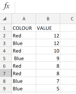 Figure 2. of Number Values in Excel.
- Make provision for a cels where Excel can return our top Values and input the formula.
In the example illustrated above, our active cell D3, will contain the following formula;
=SUMPRODUCT(LARGE((A2:A9=D3)*(B2:B9),{1.2.3.N}))
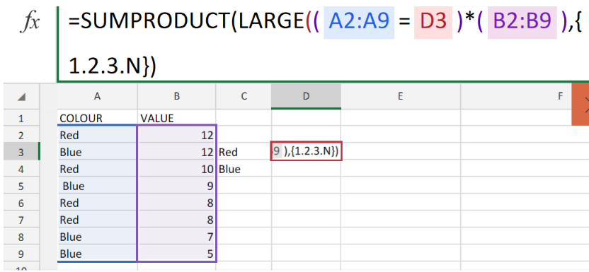 Figure 3. of LARGE and SUMPRODUCT Functions in Excel.
- Modify and copy the formula into the other criteria cell D4, to get the desired result.
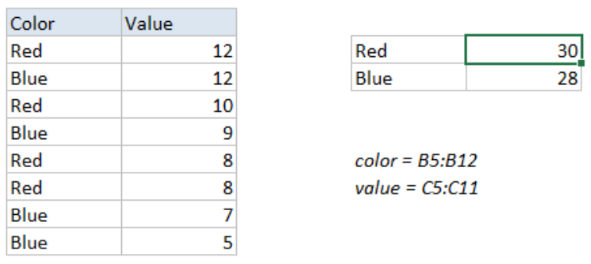 Figure 4. of Final Result..
Note
This formula operation will not match any data values in the form of text within the range of values.
Instant Connection to an Expert through our Excelchat Service
Our live Excelchat Service is here for you. We have Excel Experts available 24/7 to answer any Excel questions you may have. Guaranteed connection within 30 seconds and a customized solution for you within 20 minutes.


Leave a Comment