Sum if equal to one of many things

Excel allows a user to sum values if a cell is equal to one of many values from the other range, using the SUMPRODUCT and SUMIF functions. This step by step tutorial will assist all levels of Excel users in summing values if a cell is equal to one of many things.

Figure 1. The result of the formula

Syntax of the SUMIF Formula

The generic formula for the SUMIF function is:

=SUMIF(range, criteria_range, [sum_range])

The parameters of the SUMIF function are:

• range – a range where we want to apply our criteria
• criteria – a criteria range where we want to find a value from a range
• [sum_range] – a range which we want to sum. This is an optional parameter. If it’s omitted, the range will be summed.

Syntax of the SUMPRODUCT Formula

=SUMPRODUCT(array)

The parameter of the SUMPRODUCT function is:

• array – an array of values which we want to sum.

Setting up Our Data for the Formula

Let’s look at the structure of the data we will use. Our table consists of 3 columns: “Delivery Number” (column B), “Month” (column C) and “Amount” (column D). The criteria range is F3:F4 (“Months”). The result will be in the cell H3.

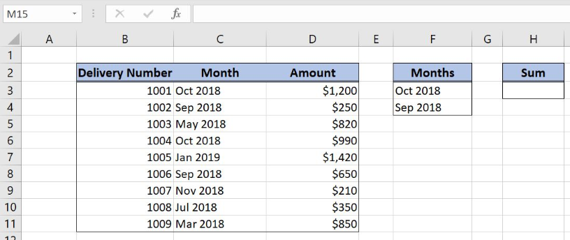Figure 2. Data that we will use in the example

Sum Amounts if a Cell is Equal to One of Many Things

In our example, we want to sum all amounts which corresponding month is Oct or Sep 2018. The result is in the cell H3.

The formula looks like:

=SUMPRODUCT(SUMIF(C3:C11, F3:F4, D3:D11))

The range of the SUMIF function is the C3:C11 range, while the criteria is F3:F4. The sum_range parameter is D3:D11. The result of the function is the array parameter of the SUMPRODUCT function. Finally, the function sums all these values.

To apply the formula, we need to follow these steps:

• Select cell H3 and click on it
• Insert the formula: =SUMPRODUCT(SUMIF(C3:C11, F3:F4, D3:D11))
• Press enter

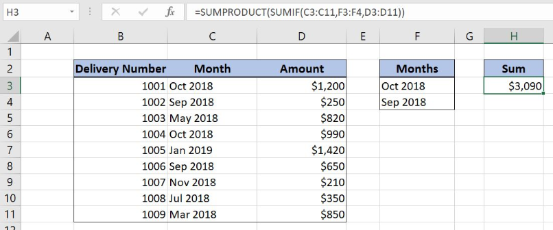Figure 3. Using the formula to sum if a cell is equal to one of many things

As we can see in Figure 3, 4 rows meet the criteria of the SUMIF function. Rows 3 and 6 have Oct 2018 and rows 4 and 8 have Sep 2018. Therefore, the result in H3 is the sum of corresponding amounts ($1,200, $990, $250 and $650) – $3,090.

Most of the time, the problem you will need to solve will be more complex than a simple application of a formula or function. If you want to save hours of research and frustration, try our live Excelchat service! Our Excel Experts are available 24/7 to answer any Excel question you may have. We guarantee a connection within 30 seconds and a customized solution within 20 minutes.