Sum If Cells Contain Specific Text

In Excel, we often need to sum cells if they contain specific text. In order to achieve this, we will use the SUMIF function which enables us to sum values from one column, while looking up for the specific text in another column. This step by step tutorial will assist all levels of Excel users in summing cells that meet a specific criteria through the use of SUMIF and Wildcards

Syntax of the SUMIF function

The generic formula for summing cells containing specific text looks like:

=SUMIF(text_range, "*specific_text*", value_range)

The parameters of the SUMIF function are:

• text_range – a range of text in which we want to find a specific text
• *specific_text* – a specific text which we want to find in text_range. An asterisk (*) is a wildcard which stands for any text. This means that we want to find a specific text even as a part of a text
• value_range – a range of values which we want to sum if the specific text is found in text_range.

Setting up Your Data

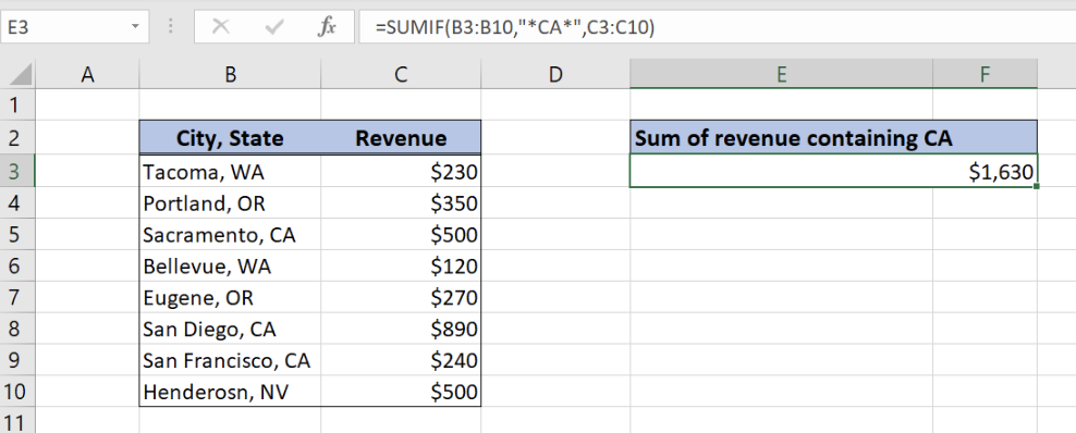Figure 1. The structure of the data

Let’s start with examining the structure of the data that we will use.

In column B (“City, State”) we have cities and states while in the column C (“Revenue”) we have revenue. In the cell E3, we want to sum all revenues which belong to California state (column B containing “CA”).

Calculate the Revenue for CA State

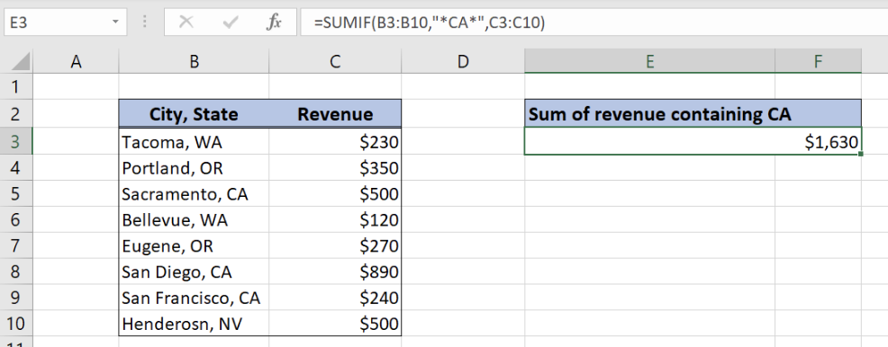Figure 2. Sum if cells contain specific text

The formula looks like:

=SUMIF(B3:B10,"*CA*",C3:C10)

In our example, text_range is “City, State” column, so the range is B3:B10. The parameter specific_text is “*CA*”, because we want to find all cells from the text range containing “CA”. Finally, value_range is “Revenue” column (the range C3:C10), which we will sum if there is “CA” in text range.

To sum all the revenues for California state, we need to follow these steps:

• Select cell E3 and click on it
• Insert the formula: =SUMIF(B3:B10,"*CA*",C3:C10)
• Press enter

As a result, we will get a value of $1,630. As we can see in the picture, the value “CA” is in cells B5, B8 and B10. Furthermore, corresponding revenues for these cells are in cells C5 ($500), C8 ($890) and C10($240). Therefore, these 3 values give a sum of $1,630 in cell E3.

Most of the time, the problem you will need to solve will be more complex than a simple application of a formula or function. If you want to save hours of research and frustration, try our live Excelchat service! Our Excel Experts are available 24/7 to answer any Excel question you may have. We guarantee a connection within 30 seconds and a customized solution within 20 minutes.