

Excel allows us to sum all values from a table that contain both x and y by using the SUMIFS function. This step by step tutorial will assist all levels of Excel users in summing values from a table with two conditions.
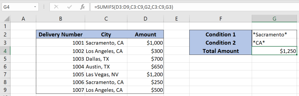 Figure 1. The final result of the SUMIFS function
Syntax of the SUMIFS formula
=SUMIFS(sum_range, criteria_range1, criteria1, criteria_range2, criteria2)
The parameters of the SUMIFS function are:
- sum_range – a range with values which we want to sum
- criteria_range1 – a range where we want to set our first condition
- criteria1 – the first condition for summing the values
- criteria_range2 – a range where we want to set our second condition
- criteria2 – the second condition for summing the values
Setting up Our Data for the SUMIFS Function
Our table consists of 3 columns: “Delivery Number” (column B), “City” (column C) and “Amount” (column D). In cells G2 and G3, we specify values that we want “City” column to contain. In the cell G4 we want to get a sum for these two conditions.
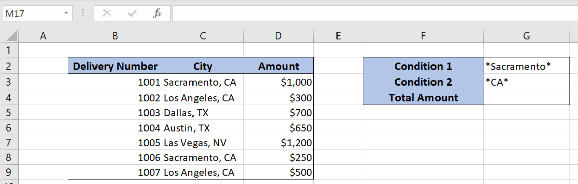 Figure 2. Data that we will use in the SUMIFS example
Sum Amount if City Contains Both Conditions
In our example, we want to sum all amounts from column D if the cells in column D contains “*Sacramento*” and “*CA*”. The asterisks (*) means that we check if the cell contains the value between them. If we put only the value then, the whole cell must match with that value.
Formula:
=SUMIFS(D3:D9, C3:C9, G2, C3:C9, G3)
The sum_range is D3:D9. Both criteria ranges are C3:C9 (“City” column) Criteria1 is G2 (“*Sacramento*”). Criteria2 is G3 (“*CA*”).
To apply the SUMIFS function, we need to follow these steps:
- Select cell G4 and click on it
- Insert the formula:
=SUMIFS(D3:D9, C3:C9, G2, C3:C9, G3) - Press enter
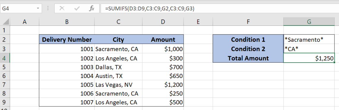 Figure 3. Using the SUMIFS function to sum values containing both conditions
In this example, we get all amounts which have “Sacramento” and “CA” in “City”. As you can see, rows 3 and 8 (Sacramento, CA) meet both conditions, so correspondings amounts are summed ($1,000 and $250). Finally, the sum in the cell G4 is $1,250.
Most of the time, the problem you will need to solve will be more complex than a simple application of a formula or function. If you want to save hours of research and frustration, try our live Excelchat service! Our Excel Experts are available 24/7 to answer any Excel question you may have. We guarantee a connection within 30 seconds and a customized solution within 20 minutes.


Leave a Comment