

When we want to add data based on a given criteria in Excel, it is best to use SUMIF or SUMIFS. This article will explain how to sum cells while looking up specific text in another cell.
 Figure 1. Final result: Sum if cell contains text in another cell
Formula using SUMIF: =SUMIF(B3:B10,"*"&"Blue"&"*",C3:C10)
Formula using SUMIFS: =SUMIFS(C3:C10,B3:B10,"*"&"Blue"&"*")
Setting up the Data
Here we have a list of orders in different colors. We want to sum the orders according to color.
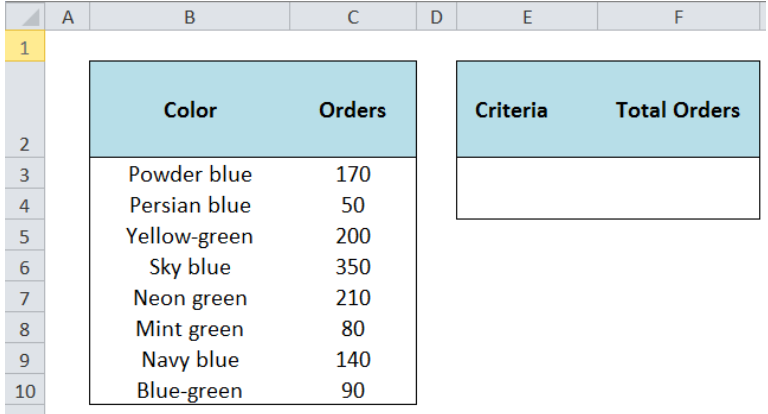 Figure 2. Sample data to sum cells based on specific text in another cell
Sum Cells in Excel
In summing cells based on the text of other cells, we can use either SUMIF or SUMIFS.
SUMIF function in Excel
SUMIF sums the values in a specified range, based on one given criteria
Syntax
=SUMIF(range,criteria, [sum_range])
Where
- Range: the data range that will be evaluated using the criteria
- Criteria: the criteria or condition that determines which cells will be added
- Sum_range: the cells that will be added; if left blank, “sum_range” = “range” which means that the range of data that will be added is the same range of data evaluated
SUMIFS function in Excel
Similar to SUMIF, SUMIFS also sums the values in a specified range, but it can be based on one or more specified criteria.
Syntax
=SUMIFS(sum_range, criteria_range1, criteria1,[criteria_range2],[criteria2]...)
- Sum_range: the cells that will be added
- Criteria_range1: the data range that will be evaluated using the criteria
- Criteria1: the criteria or condition that determines which cells will be added
- Criteria_range2 and criteria2 are optional; only applied when there are more criteria as specified
Sum If Color is Blue using SUMIF
In cell F3, enter the formula:
=SUMIF(B3:B10,"*"&"Blue"&"*",C3:C10)
This formula returns the sum of all orders in column C with any variant of color blue in column B. As shown below, the sum of 170, 50, 350, 140 and 90 is 800.
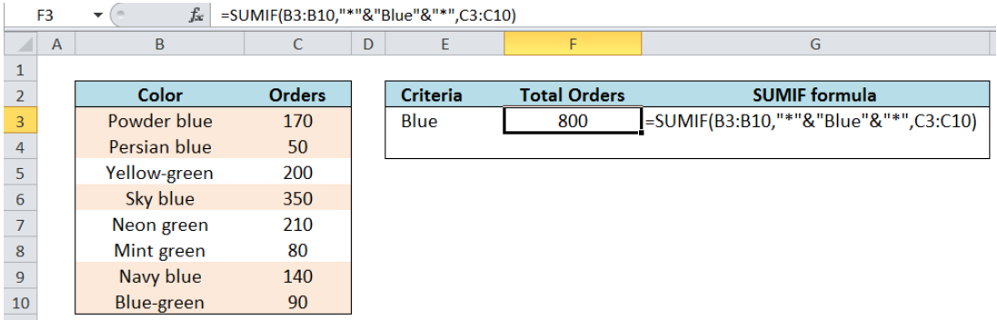 Figure 3. Entering the formula for SUMIF to sum orders of color Blue
Important Notes:
- We want to add all orders in any variant of color blue. Hence, our criteria should be *Blue* which includes all cells which may have texts before or after the word blue.
- This part of the formula: “*”&”Blue”&”*” means *Blue*
- The asterisk “ * ” is used as a wildcard in Excel, which means any number of characters
- The ampersand “&” is used to concatenate texts or strings
Alternative Formula
In cell E4, enter the text string “ *Blue* ”.
In cell F4, enter the formula:
=SUMIF(B3:B10,E4,C3:C10)
This formula also sums all orders in column C that contains the text Blue in column B. Putting asterisks in both sides of the text Blue and using *Blue* as the criteria simplifies the formula.
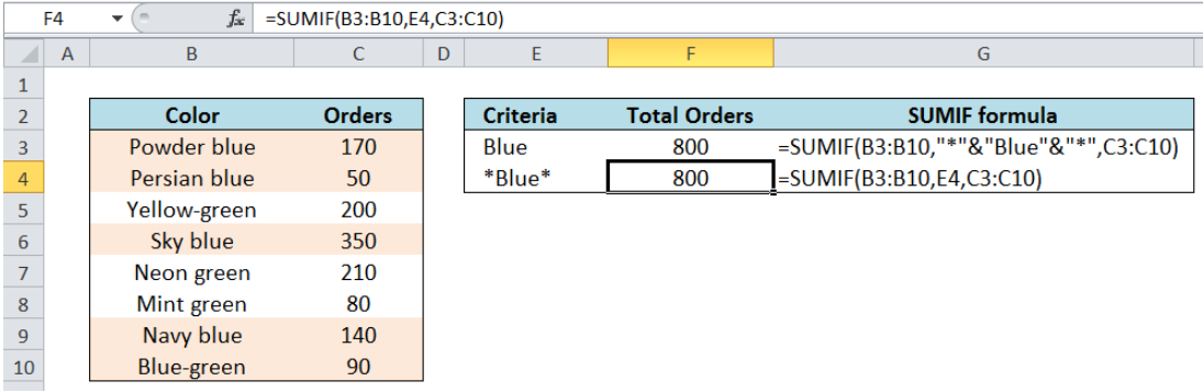 Figure 4. Simpler formula for SUMIF to sum orders of color Blue
Sum If Color is Blue using SUMIFS
In cell F3, enter the formula:
=SUMIFS(C3:C10,B3:B10,"*"&"Blue"&"*")
In cell F4, we use the alternative formula with reference to the criteria *Blue* in cell E9
=SUMIFS(C3:C10,B3:B10,E9)
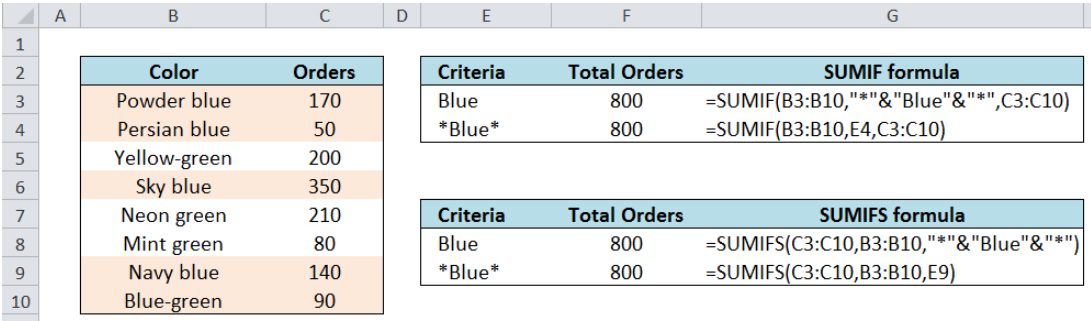 Figure 5. Comparison of SUMIF and SUMIFS in summing orders with color Blue
Both the SUMIF and SUMIFS functions return the same results. Just be mindful of the difference in syntax of these two functions. Remember, SUMIF can only be used if there is one criterion, while SUMIFS can be used with one or more criteria.
Most of the time, the problem you will need to solve will be more complex than a simple application of a formula or function. If you want to save hours of research and frustration, try our live Excelchat service! Our Excel Experts are available 24/7 to answer any Excel question you may have. We guarantee a connection within 30 seconds and a customized solution within 20 minutes.


Leave a Comment