While working with Excel, we are able to sum values that satisfy more than one criteria by using the SUMIF function. This step by step tutorial will assist all levels of Excel users in summing values by group using the IF and SUMIF functions.
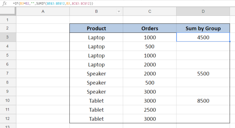
 Figure 1. Final result: Sum by group
Final formula: =IF(B3=B2,"",SUMIF($B$3:$B$12,B3,$C$3:$C$12))
Syntax of IF Function
IF function evaluates a given logical test and returns a TRUE or a FALSE
=IF(logical_test, [value_if_true], [value_if_false])
- The arguments “value_if_true” and “value_if_false” are optional. If left blank, the function will return TRUE if the logical test is met, and FALSE if otherwise.
Syntax of the SUMIF Function
SUMIF sums the values in a specified range, based on one given criteria
=SUMIF(range,criteria, [sum_range])
The parameters are:
- Range: the data range that will be evaluated using the criteria
- Criteria: the criteria or condition that determines which cells will be added
- Sum_range: the cells that will be added; if left blank, “sum_range” = “range” which means that the range of data that will be added is the same range of data evaluated
Setting up the Data
Our table has three columns: Product (column B), Orders (column C) and Sum by Group (column D). We want to group the products and calculate the sum by group. The results will be recorded in column D.
 Figure 2. Sample data to sum by group
We have three products namely: Laptop, Speaker and Tablet. First, we need to sort our data by product through these steps:
Step 1. Select the range for our data, B2:D12
Step 2. Click the Data tab, then select Create a filter
 Figure 3. Creating a filter to sort data by product
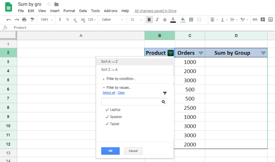
Step 3. Click the drop-down arrow for Product
Step 4. Select Sort A-Z
 Figure 4. Sorting the data by product
The resulting table will show the products arranged alphabetically.
 Figure 5. Output: Sorting the data by product through Excel filter
Sum orders by product
Now that we have sorted our data by product, we can now sum the orders per product by using the IF and SUMIF functions. Our goal is to show the sum on the first row that a product appears. Let us follow these steps:
Step 1. Select cell D3
Step 2. Enter the formula: =IF(B3=B2,"",SUMIF($B$3:$B$12,B3,$C$3:$C$12))
Step 3. Press Enter
Step 4: Copy the formula in cell D3 to cells D4:D12 by clicking the “+” icon at the bottom-right corner of cell D3 and dragging it down
Our formula evaluates if the value in B3 is equal to the value of the previous cell B2. If the logical test returns TRUE, the IF function will return an empty string ””. Otherwise, it will sum the orders in column C corresponding to the product in column B.
Since B3 “Laptop” is not equal to B2 “Product”, our formula returns the sum of orders for “Laptop”. As a result, the total orders for Laptop in cell D3 is 4500, which is the sum of 1000, 500, 1000 and 2000 in cells C3:C6.
For cells D4:D6, our formula returns as empty string “” because the value in B4:B6 is equal to the cell before it, which is Laptop.
 Figure 6. Entering the formula using IF and SUMIF to sum orders by product
For the succeeding cells in column D, our formula returns the sum of orders for “Speaker” and “Tablet” in cell D7 and D10, respectively. The cells in between are blank or empty because those are evaluated TRUE by our IF formula.
Below table shows the final result for the sum of orders per product.
 Figure 7. Output: Using IF and SUMIF to sum orders by product
Most of the time, the problem you will need to solve will be more complex than a simple application of a formula or function. If you want to save hours of research and frustration, try our live Excelchat service! Our Excel Experts are available 24/7 to answer any Excel question you may have. We guarantee a connection within 30 seconds and a customized solution within 20 minutes.


Leave a Comment