Subtotal invoices by age

Excel allows us to create subtotal for invoices by age, using the SUMIF function. This step by step tutorial will assist all levels of Excel users in creating subtotal for invoices by age.

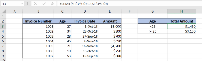Figure 1. The final result of subtotal invoices by age

Syntax of the SUMIF formula

=SUMIF(range, criteria, sum_range)

The parameters of the SUMIF function are:

• range – a range of cells which we want to evaluate
• criteria – criteria for summing data
• sum_range – a range of cells that we want to sum. This parameter is not mandatory, so if it’s omitted, a range will be summed.

Setting up Our Data for the SUMIF Function

Our table consists of 4 columns: “Delivery Number” (column B), “Age” (column C), “Invoice  Date” (column D) and “Amount” (column E). In cells H3 and H4, we want to get subtotals for the age conditions in the cells G3 and G4.

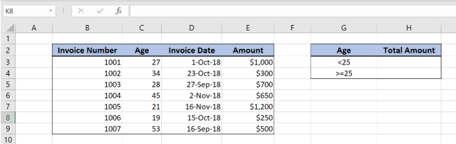Figure 2. Data that we will use in the SUMIF example

Create Subtotal of Invoices by Age

In the cell H3, we want to create the subtotal of all amounts where the age is lower than 25. All other amounts will be summed in the cell H4.

The formula looks like:

=SUMIF($C$3:$C$9, G3, $E$3:$E$9)

The range is $C$3:$C$9, while the criteria is G3. The sum_range is $E$3:$E$9. Note that we need to fix both range and sum_range, because they are not changing, only the criteria cell.

To apply the SUMIF function, we need to follow these steps:

• Select cell H3 and click on it
• Insert the formula: =SUMIF($C$3:$C$9, G3, $E$3:$E$9)
• Press enter
• Drag the formula down to the other cells in the column by clicking and dragging the little “+” icon at the bottom-right of the cell.

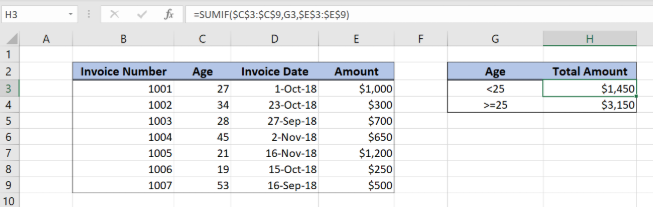Figure 3. Using the SUMIF function to create subtotals by age

As we can see in Figure 3, rows 7 and 8 have age lower than 25, so corresponding amounts are summed ($1,200 and $250). Therefore, the result of the SUMIF function in the cell H3 is $1,450.

Most of the time, the problem you will need to solve will be more complex than a simple application of a formula or function. If you want to save hours of research and frustration, try our live Excelchat service! Our Excel Experts are available 24/7 to answer any Excel question you may have. We guarantee a connection within 30 seconds and a customized solution within 20 minutes.