
Excel allows us to get a rank of a value in a list, using the PERCENTRANK function. The rank presents a percentage of values which are lower than a selected value. This step by step tutorial will assist all levels of Excel users in finding a relative position of a value in a list.
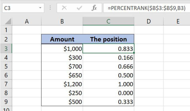 Figure 1. The final result of the PERCENTRANK function
Syntax of the PERCENTRANK formula
=PERCENTRANK(array, x, [significance])
The parameters of the PERCENTRANK function are:
- array – a list of values
- x – a value from the list for which we want to find the position
- [significance] – a number of decimal digits of the result. This is the non-mandatory parameter and if omitted, it will be 3.
Setting up Our Data for the PERCENTRANK Function
In column B (“Amount”), we have the list of values. In column C (“The position”), we want to get a relative position for each value in the list.
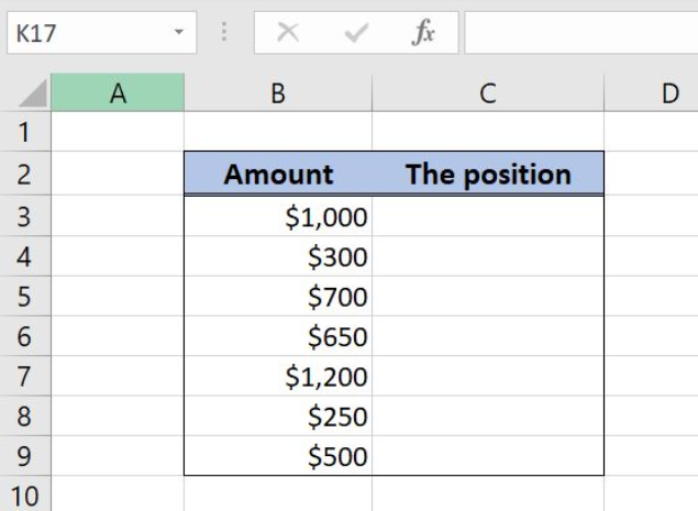 Figure 2. Data that we will use in the PERCENTRANK example
Find a Relative Position of Values in the List
In the cell C3, we want to get a relative position of the cell B3. In other words, we want to find out the percentage of values which are lower than $1,000.
The formula looks like:
=PERCENTRANK($B$3:$B$9, B3)
The array is $B$3:$B$9, while the x is B3. Note that we need to fix the array, as it’s not changing, only the x cell.
To apply the PERCENTRANK function, we need to follow these steps:
- Select cell C3 and click on it
- Insert the formula:
=PERCENTRANK($B$3:$B$9, B3) - Press enter
- Drag the formula down to the other cells in the column by clicking and dragging the little “+” icon at the bottom-right of the cell.
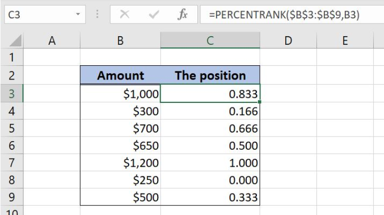 Figure 3. Using the PERCENTRANK function to find a relative position of a value
As we can see, there are 7 values in column B and $1,000 is greater than 5 of them. That means it’s greater than ⅚ value, which is 0.833. This percentage is the result of the function in the cell C3.
Most of the time, the problem you will need to solve will be more complex than a simple application of a formula or function. If you want to save hours of research and frustration, try our live Excelchat service! Our Excel Experts are available 24/7 to answer any Excel question you may have. We guarantee a connection within 30 seconds and a customized solution within 20 minutes.


Leave a Comment