Last row in mixed data with blanks

Excel allows us to get the last row in mixed data with blanks using the MATCH function. This step by step tutorial will assist all levels of Excel users in getting the last row in mixed data with blanks.

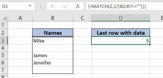Figure 1. The result of the MATCH function

Syntax of the MATCH Formula

=MATCH(lookup_value, lookup_array, [match_type])

The parameters of the MATCH function are:

• lookup_value – a value which we want to find in the lookup_array
• lookup_array – the array where we want to find a value
• [match_type] – a type of match. This is an optional parameter and if it’s omitted, the value is 1 – approximate match.

Setting up Our Data to Get Excel Table Column Number

In the range B2:B7 we have the array of names. In the cell D3, we want to get the last row from this range that is not blank.

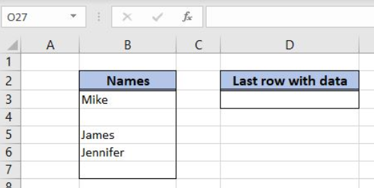Figure 2. The data structure for the MATCH example

Getting the Last Row in Mixed Data with Blanks Using the MATCH Function

We want to get the last populated row in the range B2:B7 in the cell D3.

The formula looks like:

{=MATCH(2, 1/(B2:B7<>""))}

The lookup_value in the MATCH function is 2. The lookup_array is 1/(B2:B7<>””). The B2:B7<>”” will return the array of TRUE and FALSE values. Excel interprets these values as 1 and 0. After that, the function will divide 1 with all these values and get 1 or division by zero error. As we want to find 2 in this array and there will never be 2, the function will return the last 1 as the appropriate match.

To apply the MATCH function we need to follow these steps:

• Select cell D3 and click on it
• Insert the formula: =MATCH(2, 1/(B2:B7<>""))
• Press Ctrl+Shift+Enter, because this is the array formula.

Figure 3. Get the last row in mixed data with blanks using the MATCH function

When we evaluate the formula, we can see that in the first step it looks like this:

=MATCH(2,1/({TRUE,TRUE,FALSE,TRUE,TRUE,FALSE})

In the next step, this is the situation:

=MATCH(2,{1,1,#DIV/0!,1,1,#DIV/0!})

Finally, there is no 2 in the lookup array, so the approximate match is the last 1 in the array. Therefore, the result in D3 is 5.

Most of the time, the problem you will need to solve will be more complex than a simple application of a formula or function. If you want to save hours of research and frustration, try our live Excelchat service! Our Excel Experts are available 24/7 to answer any Excel question you may have. We guarantee a connection within 30 seconds and a customized solution within 20 minutes.