Using Excel to Calculate Random Number Weighted Probability

Excel can return a value randomly based on its probability by using SUM, MATCH and RAND functions. This step by step tutorial will assist all levels of Excel users in randomly creating a list of values based on their probability of being selected.

The Final Formula:

=match(rand(),$C$2:$C$6)

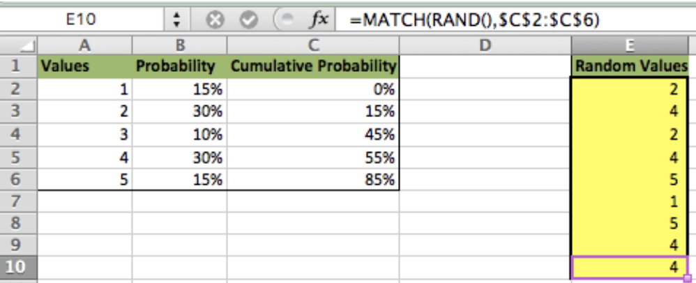Figure 1. Random value generation using MATCH and RAND functions

Creating a Cumulative Probability

• First, we setup our data so that we have the value to be returned in Column A, the probability in Column B and a blank Column C
• In cell C2, we type “0”. In cell C3, we type this formula =sum(B1,C1) and copy the formula down to the bottom of our data
• Notice how we purposely offset the formula by 1 row. This is because 0 starts the range between 0 and 1, so the first value in Column C must equal zero. Then, the rest of the cells in column C will add the previous percentages together to form percentage increments which represents the probability that each value will be selected
• Take the difference between 85% and 55% which equals 30%. This is the specified probability of Value 4 being selected

Figure 2. Random value generation using MATCH and RAND functions

Now that we have the cumulative probability created and we are familiar with the MATCH function, we can now use the RAND function to generate a list of random numbers between 0 and 1 and find the closest lower match of the random number. See below

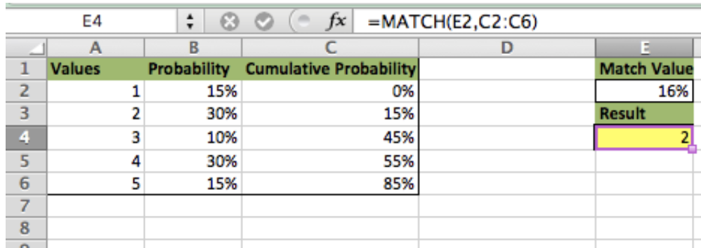
Lookup Value Using MATCH Function

The match function returns the ROW in which the closest data match is found. We can use the MATCH function to find the value that is within the probability range. In order to complete this task using other data, we will need to use the INDEX function which will be explained later in the article

MATCH Function Syntax:

=MATCH(Lookup Value, Lookup Table Array, Approximate Match [True/False])

• Enter the lookup probability in cell E2
• In cell E4 type this formula
  =match(E2,C2:C6)
• In this example the formula returned Value 2 because 16% is between 15% and 45%. Once the value in cell E2 is 45% or greater, the new returned value in E4 would become Value 3 and so forth

Note: This will only work if the data is numbered in sequence with the number of values available. Therefore, if this was five rows of data, the values would have to be 1, 2, 3, 4 and 5 in ascending order. For other types of data, we will need to use the INDEX function explained later in the article.

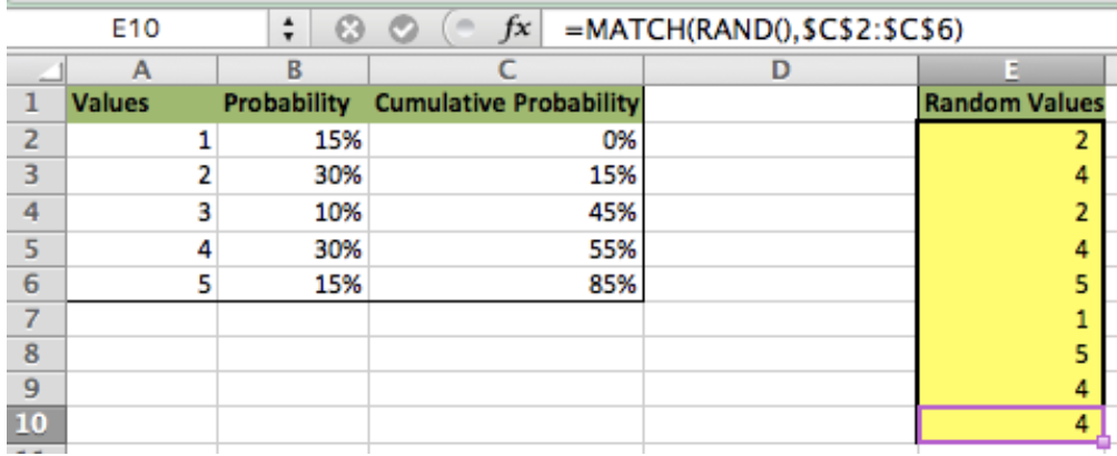
*The previous series of steps were used to illustrate how the match function looks up data. In the next series of steps we will generate multiple random values in column E by adding RAND to our MATCH formula to generate a more dynamic matching function.

Lookup Value Using RAND Function

The RAND function returns a random value between 0 and 1. We will use the RAND function to develop the random lookup.

• In cell E2 type this formula
  =MATCH(RAND(),$C$2:$C$6)
• Be sure to create absolute references (by using the ‘$’ sign) on your data array and copy the formula down to cell E10
• The formula returns the matching ROW value from column A based on the ROW where Column C matches the random number

Bonus Step:

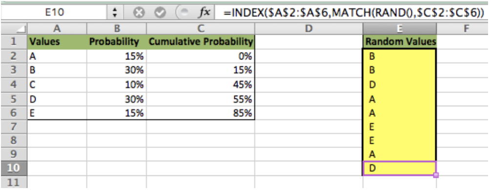
If your value list is Text instead of numbers or is not numbered in sequence with the data, you can add the INDEX function to the formula to randomly lookup the text value based on its probability

Lookup Text Value Using Index Function

• The INDEX function returns a value based on the ROW and COLUMN the user specifies  – Example: “=Index(1,1)” returns the value in cell A1 (ROW 1, COLUMN 1)
• We can use this concept to find the matching row by nesting the INDEX, MATCH and RAND functions
• In cell E2 type this formula
  =INDEX($A$2:$A$6,MATCH(RAND(),$C$2:$C$6))
• The formula returns the text value in column A based on it’s probability of being selected
• Be sure to create absolute references on your data arrays and copy the formula down to cell E10

Instant Connection to an Expert through our Excelchat Service:

Most of the time, the problem you will need to solve will be more complex than a simple application of a formula or function. If you want to save hours of research and frustration, try our live Excelchat service! Our Excel Experts are available 24/7 to answer any Excel question you may have. We guarantee a connection within 30 seconds and a customized solution within 20 minutes.