

Excel allows us to set up an electronic raffle using the RAND, INDEX, MATCH and MAX functions. This step by step tutorial will assist all levels of Excel users to get the random winner in the electronic raffle.
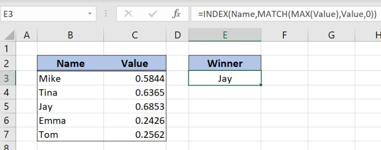 Figure 1. The final result of the formula
Syntax of the RAND Formula
The generic formula for the RAND function is:
=RAND()
The function returns a random decimal number between 0 and 1 and has no parameters.
Syntax of the INDEX Formula
The generic formula for the INDEX function is:
=INDEX(array, row_num, column_num)
The parameters of the INDEX function are:
- array – a range of cells where we want to get a data
- row_num – a number of a row in the array for which we want to get a value
- column_num – a column in the array which returns a value.
Syntax of the MATCH Formula
The generic formula for the MATCH function is:
=MATCH(lookup_value, lookup_array, [match_type])
The parameters of the MATCH function are:
- lookup_value – a value which we want to find in the lookup_array
- lookup_array – the array where we want to find a value
- [match_type] – a type of match. We put 0 which is an exact match.
Syntax of the MAX Formula
The generic formula for the MAX function is:
=MAX(number1, [number2], ...)
The parameters of the MAX function are:
- number1, [number2] – the numbers from which we want to get the maximum values
Setting up Our Data for the Electronic Raffle
Our table consists of 2 columns: “Name” (column B) and “Value” (column C). In column “Value” will be placed random numbers from 0 to 1 that will help us in the calculation. The second table has an empty cell E3 where we will get the winner name of the electronic raffle.
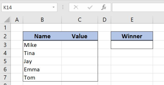 Figure 2. Data for the electronic raffle
Set Up an Electronic Raffle with Excel Functions
We want to get the random name from column B and to place the result in the cell E3. In order to make the formula more clear, we will create a named range Name for cell range B3:B7 and a named range Value for the cell range C3:C7.
To create a named range we should follow the steps:
- Select the cell range that should be named
- Click on the name box in Excel
- Write the name for the cell range and press enter
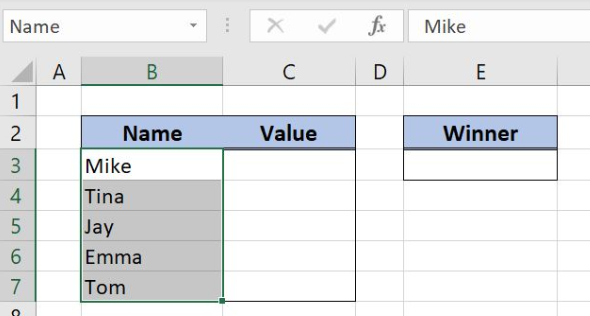 Figure 3. Creating a named range Name for column “Name”
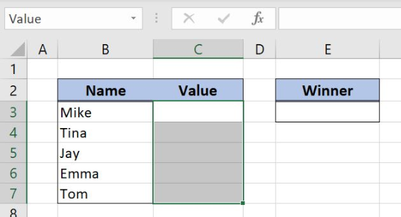 Figure 4. Creating a named range Value for column “Value”
The formula in Column C looks like:
=RAND()
The RAND function gets the random value from 0 to 1. The randomized values are placed in column C and will help us to get the winner in the electronic raffle.
To apply the formula, we need to follow these steps:
- Select cell C3 and click on it
- Insert the formula:
=RAND() - Press enter.
- Drag the formula down to the other cells in the column by clicking and dragging the little “+” icon at the bottom-right of the cell.
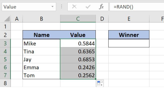 Figure 5. Using the RAND formula to get a random value between 0 and 1
Now we can place the formula in the cell E3 to get the winner of the electronic raffle:
=INDEX(Name,MATCH(MAX(Value),Value,0))
The parameter array in the INDEX function is a named range Name while the row_num is the formula MATCH(MAX(Value),Value,0). In the MATCH function, lookup_value is a formula MAX(Value) while the parameter lookup_array is the named range Value. A match_type is 0 because we want the exact match. Finally, the parameter number1 in the MAX function is the named range Value.
To apply the formula, we need to follow these steps:
- Select cell E3 and click on it
- Insert the formula:
=INDEX(Name,MATCH(MAX(Value),Value,0)) - Press enter.
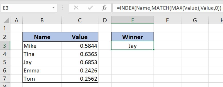 Figure 6. Get the winner of the electronic raffle with RAND, INDEX, MATCH and MAX functions
With MAX function we get the maximum value from column “Value”. The MATCH function searches maximum value in the column “Value” and retrieves the position of that value in the named range Value. The INDEX function gets the name from column B based on the MATCH function result, the row number 3. As a result, the winner of the electronic raffle is Jay.
Most of the time, the problem you will need to solve will be more complex than a simple application of a formula or function. If you want to save hours of research and frustration, try our live Excelchat service! Our Excel Experts are available 24/7 to answer any Excel question you may have. We guarantee a connection within 30 seconds and a customized solution within 20 minutes.


Leave a Comment