

Excel allows us to generate unique random numbers in Excel using the RAND and RANK functions. This step by step tutorial will assist all levels of Excel users to find out how to generate unique random numbers in Excel.
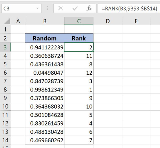 Figure 1. The final result of the formula
Syntax of the RAND Formula
The generic formula for the RAND function is:
=RAND()
The function returns a random decimal number between 0 and 1 and has no parameters.
Syntax of the RANK Formula
The generic formula for the RANK function is:
=RANK(number, ref, [order])
The parameters of the RANK function are:
- number – a number which we want to rank
- ref – a list of numbers for ranking
- [order] – 1 for ascending or 0 for descending order. This parameter is optional, if it’s omitted, the default order is descending.
Set up a Random Team Generator
First, we need to get a random number in column B
The formula for RAND in B3 looks like:
=RAND()
To apply the formula, we need to follow these steps:
- Select cell B3 and click on it
- Insert the formula:
=RAND() - Press enter
- Drag the formula down to the other cells in the column by clicking and dragging the little “+” icon at the bottom-right of the cell.
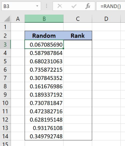 Figure 2. Using the RAND formula
When we get a random number we can rank them in column C.
The formula for RANK in C3 looks like:
=RANK(B3, $B$3:$B$14)
The number parameter is the cell B3. The ref parameter is the range $B$3:$B$14. We must fix the range, as it’s not changing when the formula is copied down the cells.
To apply the formula, we need to follow these steps:
- Select cell C3 and click on it
- Insert the formula:
=RANK(B3,$B$3:$B$14) - Press enter
- Drag the formula down to the other cells in the column by clicking and dragging the little “+” icon at the bottom-right of the cell.
![]() Figure 3. Using the RANK formula
Figure 3. Using the RANK formula
Now we have 12 unique random numbers in column C.
Most of the time, the problem you will need to solve will be more complex than a simple application of a formula or function. If you want to save hours of research and frustration, try our live Excelchat service! Our Excel Experts are available 24/7 to answer any Excel question you may have. We guarantee a connection within 30 seconds and a customized solution within 20 minutes.


Leave a Comment