

Pivot tables, by default, cannot be automatically refreshed. While working with Excel, we can manually refresh our pivot table every time we make some changes in the source data. This step by step tutorial will assist all levels of Excel users in refreshing a pivot table in Excel.
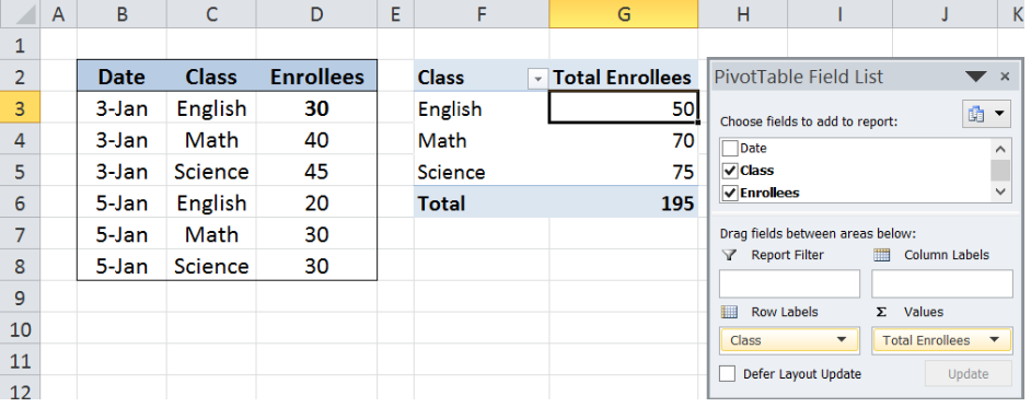 Figure 1. Final result: Refresh a pivot table in Excel
Setting up Our Data
Our source table contains three columns: Date (column B), Class (column C) and Enrollees (column D).
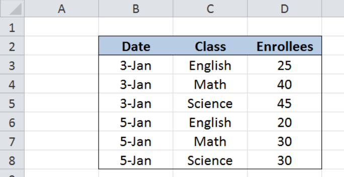 Figure 2. Sample data to refresh a pivot table in Excel
We use above data to create a pivot table showing the total enrollees per class.
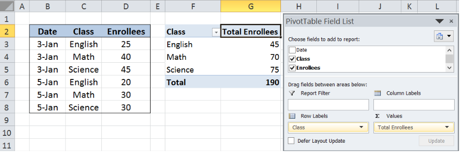 Figure 3. Pivot table created from the source data
Next we make some changes to our source data. Suppose we need to correct the value in cell D3 and change the number of enrollees from 25 to 30. Note that our pivot table does not automatically change with our data. The total enrollees for English in our pivot table is still 45 instead of 50.
 Figure 4. Pivot table data remains unchanged after changing the value of D3
Refresh pivot table manually
We can refresh a pivot table anytime in Excel by clicking the Refresh button. To refresh a pivot table manually, let us follow these steps:
Step 1. Click the Options tab
Step 2. Click Refresh. We can also click Refresh All to update all workbooks at once
 Figure 5. Refresh button to update pivot table data
Our pivot table is instantly updated to include the changes we made to our source table. The total enrollees for English is now changed from 45 to 50, as shown in cell G3.
 Figure 6. Pivot table data updated after clicking Refresh button
Note:
Excel has built-in shortcut keys for Refresh and Refresh All. For Refresh, just press Alt + F5. For Refresh All, press Ctrl + Alt + F5.
Refresh pivot table automatically when opening the workbook
There is an option in Excel where we can set our pivot table data to automatically refresh every time the workbook is opened. Let us follow these steps:
Step 1. Click the Options tab
Step 2. Select PivotTable Options
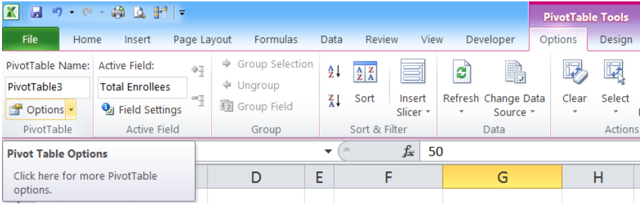 Figure 7. PivotTable options in Excel under Options tab
Step 3. In the PivotTable Options dialog box, click the Data tab, and tick Refresh data when opening the file
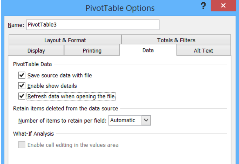 Figure 8. Setting the pivot table data to refresh when opening the file
Step 4. Click OK.
After clicking OK, Excel might show below warning message when we have other pivot tables created from the same source data. Just click OK.
 Figure 9. Warning message for multiple pivot tables created from the same source data
Now everytime we close and open the workbook, our pivot table is automatically updated to include the changes we made to our source table, including external data sources.
Most of the time, the problem you will need to solve will be more complex than a simple application of a formula or function. If you want to save hours of research and frustration, try our live Excelchat service! Our Excel Experts are available 24/7 to answer any Excel question you may have. We guarantee a connection within 30 seconds and a customized solution within 20 minutes.


Leave a Comment