

We can use a variety of ways to Sort our data in a PivotTable. This helps us to analyze, summarize and calculate data based on priority. It also enables us to visualize trends, comparisons, and patterns in our data. The steps below will walk through the process.
 Figure 1- How to Sort Pivot Table Data in Excel
Setting up the Data
- We will use the created Pivot table to sort the data
 Figure 2 – Setting up the Data
Sorting the Pivot Table Data from Recent date to older dates
- We will click on any date within the Pivot Table
- We will right-click and click on Sort
- We will select Newest to oldest
 Figure 3- Recent date to older dates
- We can do the converse for older dates to recent dates
Using the Data tab option
We can also use the data tab option to sort the dates based on our preferences. However, we will use it to sort the Sales Amount from the highest to the lowest Sales Amount.
- We will click any of the Sales Amount in the Pivot Table
- We will click on DATA and click on Sort below it
 Figure 4- Clicking the Data Tab
- We will select Largest to Smallest and click OK
 Figure 5- Sorting the highest Sales Amount to the lowest Sales Amount
 Figure 6- Highest to Lowest Sales Amount
More Sort Options
- We will click on any cell within the Pivot Table
- We will right-click and click on Sort
- We will click on more sort options
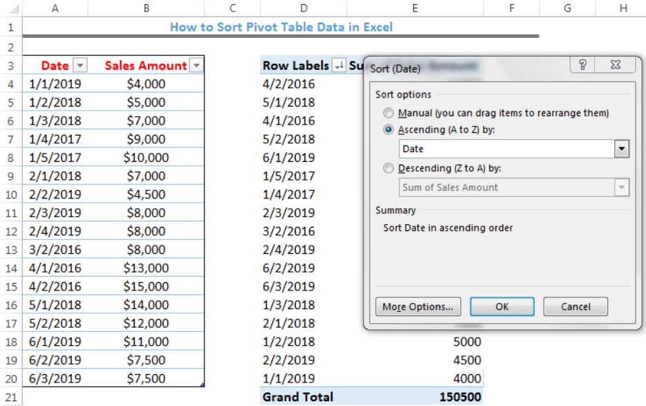 Figure 7- More sort Options
- The parameters we have picked mean that the dates will be sorted from the oldest dates to the recent dates.
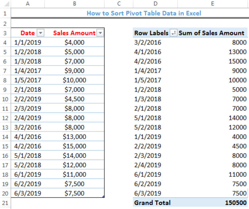 Figure 8- More sort Options
Instant Connection to an Expert through our Excelchat Service
Most of the time, the problem you will need to solve will be more complex than a simple application of a formula or function. If you want to save hours of research and frustration, try our live Excelchat service! Our Excel Experts are available 24/7 to answer any Excel question you may have. We guarantee a connection within 30 seconds and a customized solution within 20 minutes.


Leave a Comment