

We can use the Pivot table to summarize data efficiently. The Pivot table is one of the most powerful and exciting tools in Excel. In this Pivot tutorial, we will learn how to use them seamlessly.
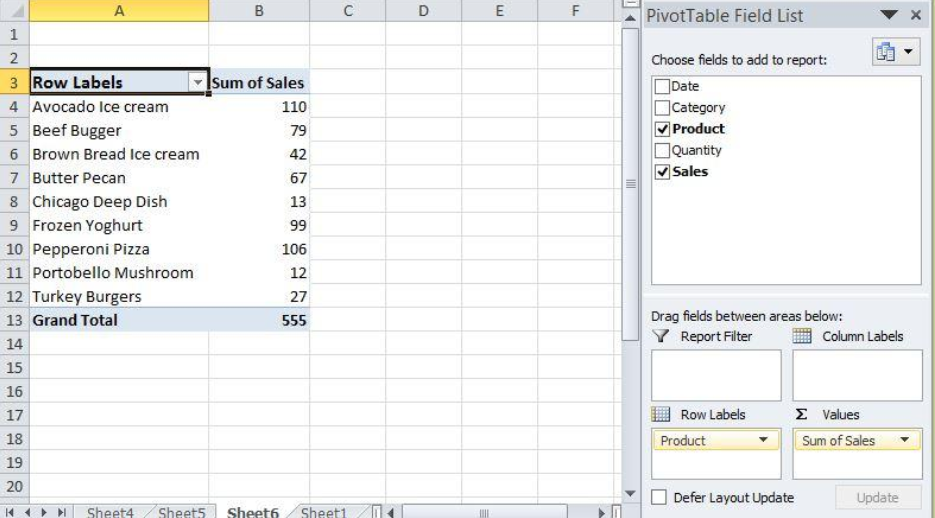 Figure 1 – Example of a simple pivot table
What is a Pivot table?
We use the Pivot table to achieve a summary of our data, displayed in an organized table which is easy to understand and make reports. We do not use Pivot tables to add or remove data.
If we want to sort, count, total or average our data, pivot tables can provide a swift pathway. There are many more ways we can customize, tweak, or visualize our data when using pivot tables.
How to Set up a Simple Pivot Table
We can create a Pivot table in one minute; it is the fastest way to organize our data without errors.
- We will enter our data in an array of rows and columns
 Figure 2- Set up data in rows and columns
- We will select any cell in our source data
- We will click the Insert tab, and then, the Pivot table button
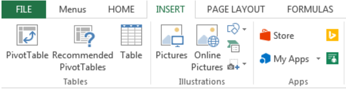 Figure 3- Clicking on Pivot Table
- In the Create Pivot table dialog box, we will check the boxes as shown below and select OK
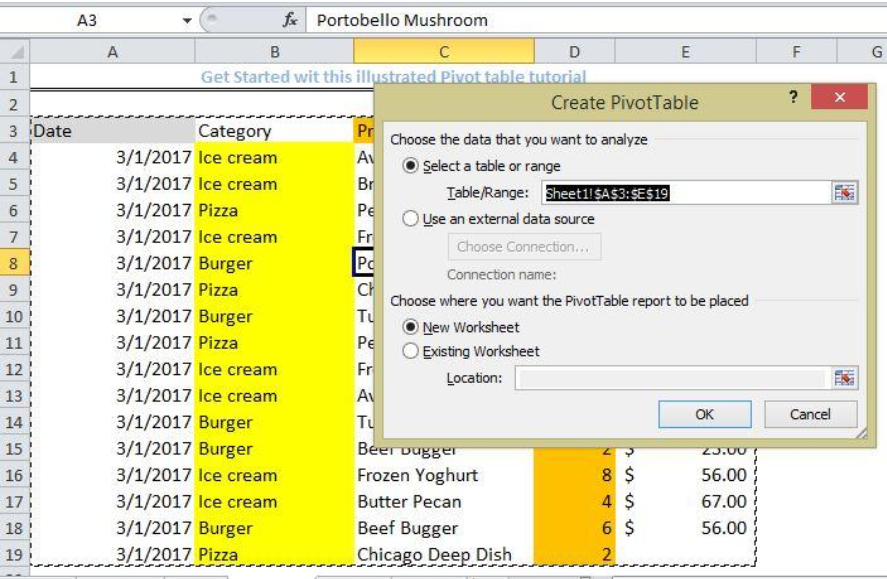 Figure 4 – Create Pivot Table dialog box
- We will click OK
- We will drag a “label” field into the Rows Labels area (for example, Product)
- We will drag a numeric field into the values area (for example, Sales)
 Figure 5 – Getting started with a simple pivot tutorial
How to use a Pivot table
Use Pivot Tables to Count Things
- We can take a count by clicking on the drop-down arrow of the Values section in the Pivot Table Field List
- We will click on Value Field Settings and Select Count as shown in figure 6
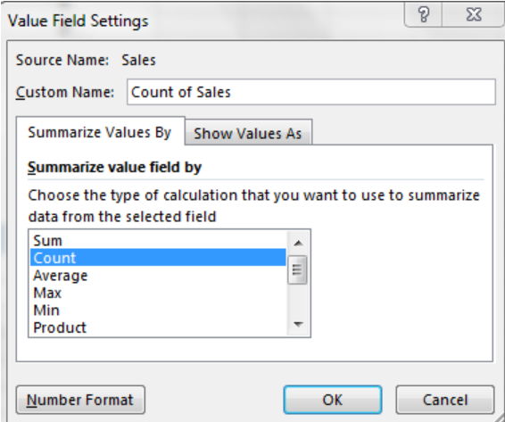 Figure 6- Value Field Settings
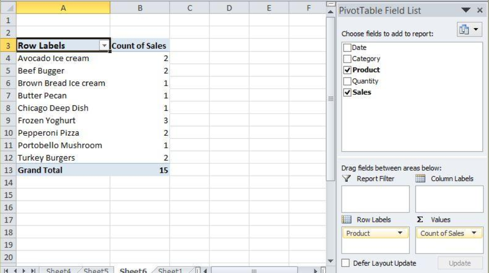 Figure 7 – Using a Pivot table to count things
Show Totals as a percentage
- We can show the count of sales in figure 7 as a percentage with the value field settings
- We will click on show value as and select % of Column Total
- We will press OK
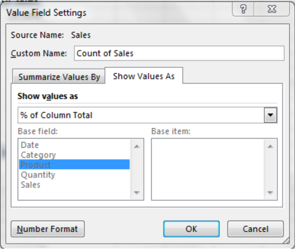 Figure 8- show values as % of Column Total
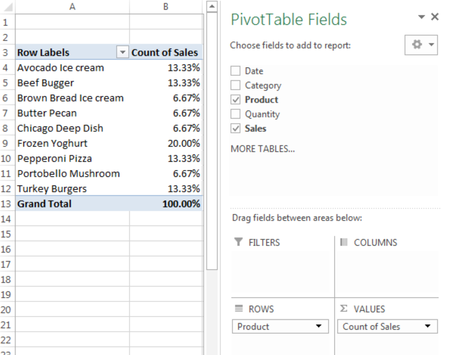 Figure 9 – Using Pivot table to get a count of sales as a percentage
Grouping our data
We can group our data in a custom way. For example, if our data sheet has several dates, we can group it into days, months, etc.
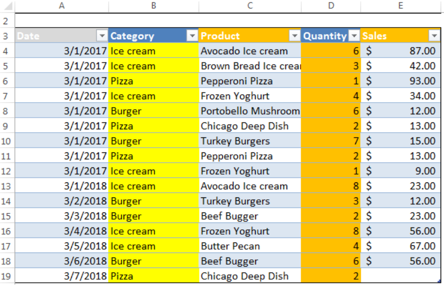 Figure 10 – Data with different Dates
- After creating the Pivot table, we will right-click on any of the dates, click on group and select the parameter to group with
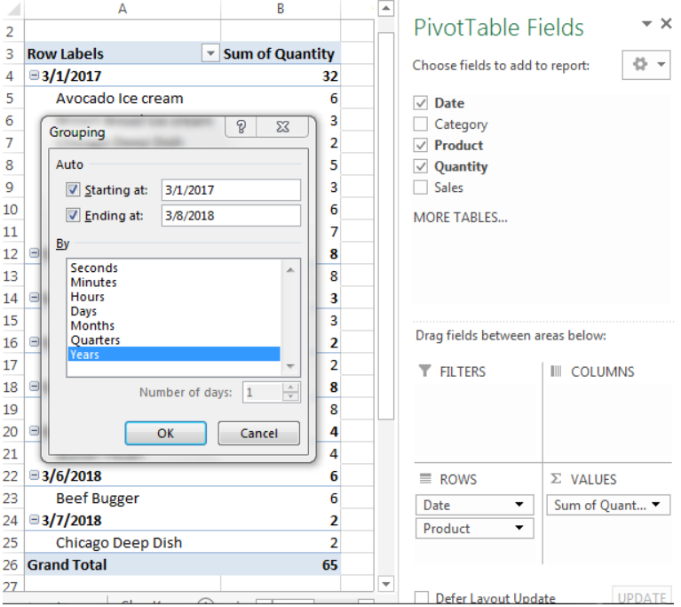 Figure 11 – Grouping Dialog box
- We will click OK
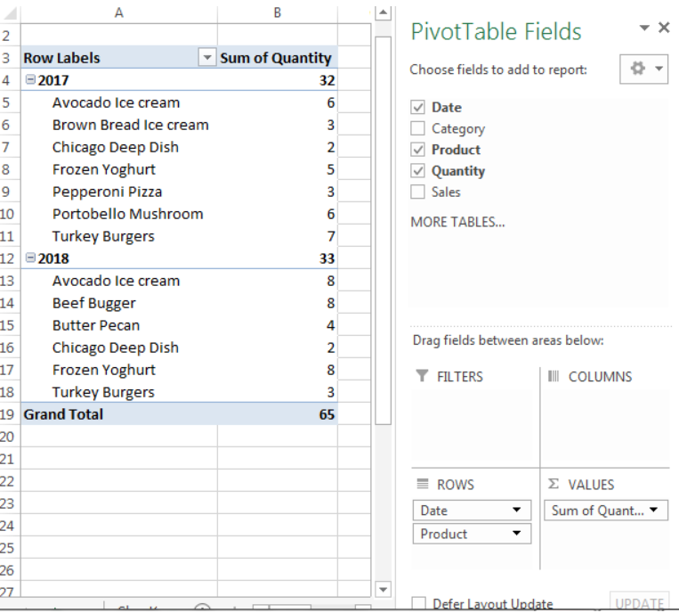 Figure 12– Pivot Table grouped by Year
Dealing with blank cells
When we have blank spaces in our data, we can customize our pivot table to fill these empty cells with a default value such as “$0” or “TBD (To Be Determined).”
- We will click on options
- For 2013 Excel, we will click Analyze to find options at the far left
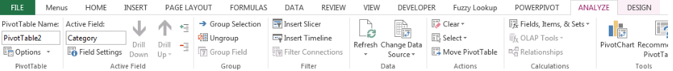 Figure 13– Pivot Table options
![]() Figure 14 – Dealing with blank cells
Figure 14 – Dealing with blank cells
![]() Figure 15 – Using Pivot table to handle empty cells
Figure 15 – Using Pivot table to handle empty cells
Instant Connection to an Expert through our Excelchat Service
Most of the time, the problem you will need to solve will be more complex than a simple application of a formula or function. If you want to save hours of research and frustration, try our live Excelchat service! Our Excel Experts are available 24/7 to answer any Excel question you may have. We guarantee a connection within 30 seconds and a customized solution within 20 minutes.


Leave a Comment