

We can insert subtotal amounts to a data in a PivotTable. This enables us to analyze, summarize, calculate, and visualize trends, comparisons, and patterns in our data. The steps below will walk through the process.
 Figure 1: How to Calculate a Subtotal in an Excel Pivot Table
Setting up the Data
- We will find calculate subtotals for the marketers based on their SALES FIGURES and ORDERS
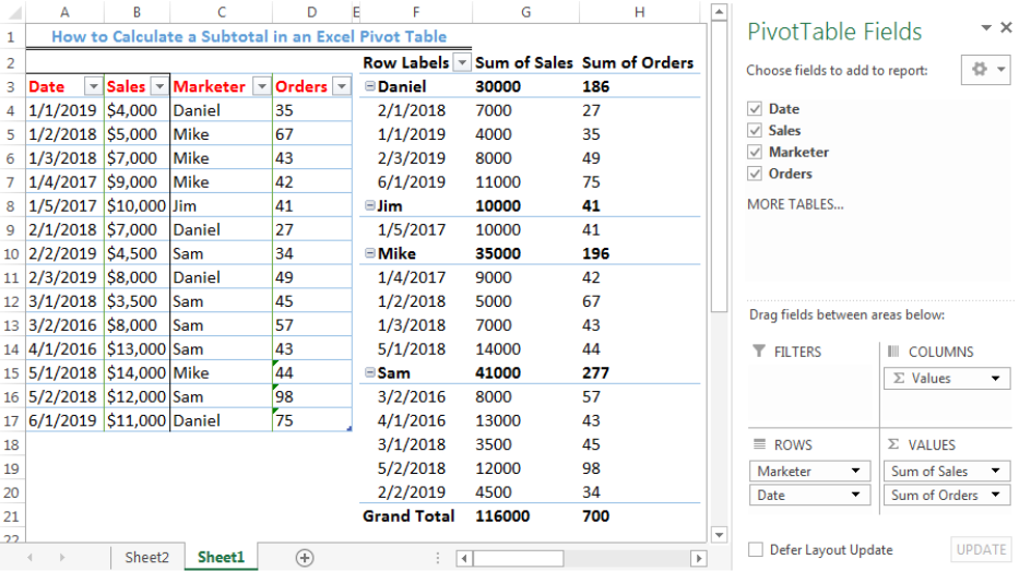 Figure 2: Setting up the Data
Subtotal For Average
- We will use Subtotal to find the average sales and order for each marketer
- We will click on any of the marketers in the Row Labels, e.g. Daniel
- We will right-click and click on field settings
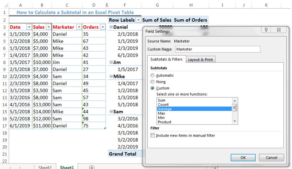 Figure 3: Field Settings Dialog box
- We will click check the Custom box and select Average as the function
- We will press OK
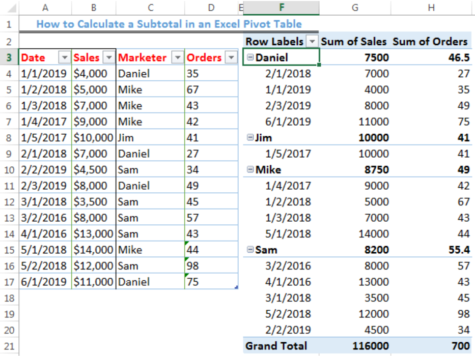 Figure 4- Result of Using Subtotal Showing Average Sum of Sales and Orders
Subtotal For Average and Maximum Sales and Orders per Marketer
- We will follow the same process up to field settings and select Average and Max
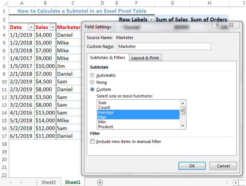 Figure 5: Field Settings Dialog Box
- We will click OK
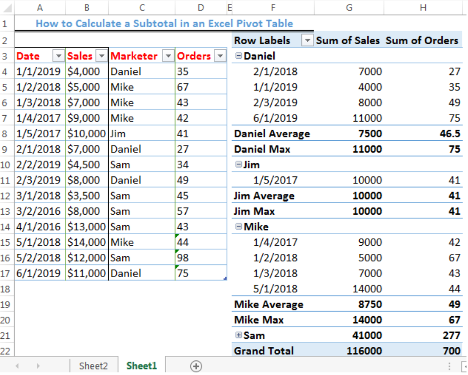 Figure 6: Result of Subtotal For Average and Maximum Sales and Orders per Marketer
Instant Connection to an Expert through our Excelchat Service
Most of the time, the problem you will need to solve will be more complex than a simple application of a formula or function. If you want to save hours of research and frustration, try our live Excelchat service! Our Excel Experts are available 24/7 to answer any Excel question you may have. We guarantee a connection within 30 seconds and a customized solution within 20 minutes.


Leave a Comment