

We can use the Power Pivot Add-In in Excel to create a pivot table from multiple workbooks. The steps below will walk through the process of creating a Pivot Table from Multiple Workbooks.
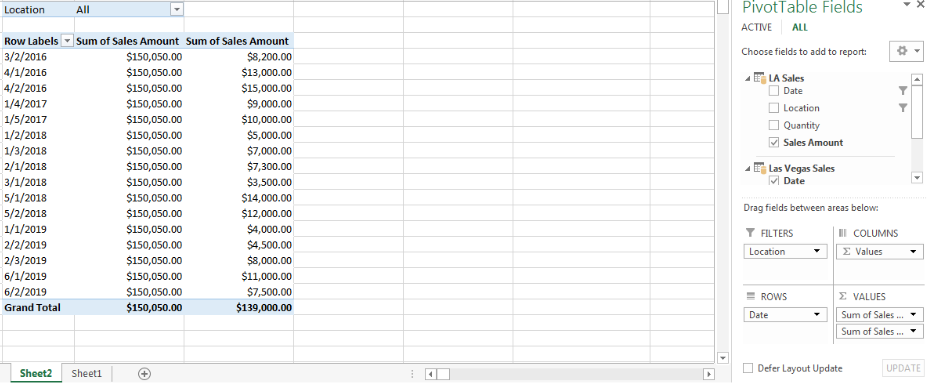 Figure 1- How to Create a Pivot Table from Multiple Workbooks
Setting up the Data
- We will open a New excel sheet and insert our data. We must put the data in a table form. We will click on any cell in the table, click on the Insert tab, click on Table, and click OK on the resulting dialog box. Click on the Table name box to name the table. We will save the excel sheet in a location in our computer
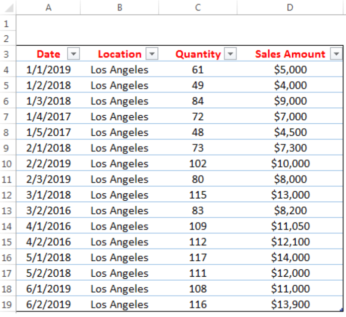 Figure 2- Setting up the Data
- We will have a similar sheet with the same Headers for Las Vegas location
Creating a Connection
- We will open a new excel sheet
- On the Data tab, we will click on Connections
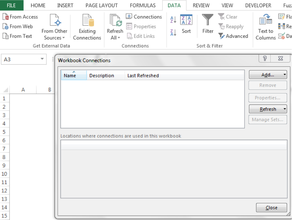 Figure 3- Creating Connections
- We will on Add
 Figure 4- Creating Connections
- We will click on Browse for More to locate the worksheet in our computer
 Figure 5- Connection Dialog Box
- Once we have located the workbook and clicked on it, the dialog box in figure 5 will appear. We will click on OK and then, close
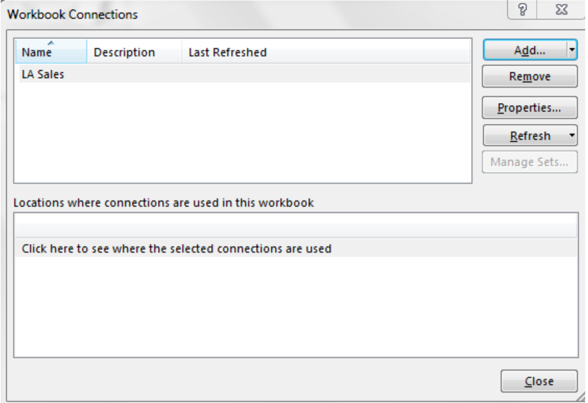 Figure 6- Los Angeles Workbook connection added
- We will go through the same process to add the second or more workbooks to connection. Here, our second workbook is Titled “Las Vegas Sales”
Using the Power Pivot Add-In
- We will click on Power Pivot and click on Manage
 Figure 7- Using the Power Pivot Add-In
- We will click on Get external data
 Figure 8- Using the Power Pivot Add-In
- We will click on existing connection and select the connected workbook
 Figure 9- Adding Los Angeles Sales Workbook
- We will click on open and click on next in figure 10
 Figure 10- Table import wizard
- We can change the Friendly name to whatever we want and click on finish
 Figure 11- Table import wizard
- We can rename any column that doesn’t have the column header
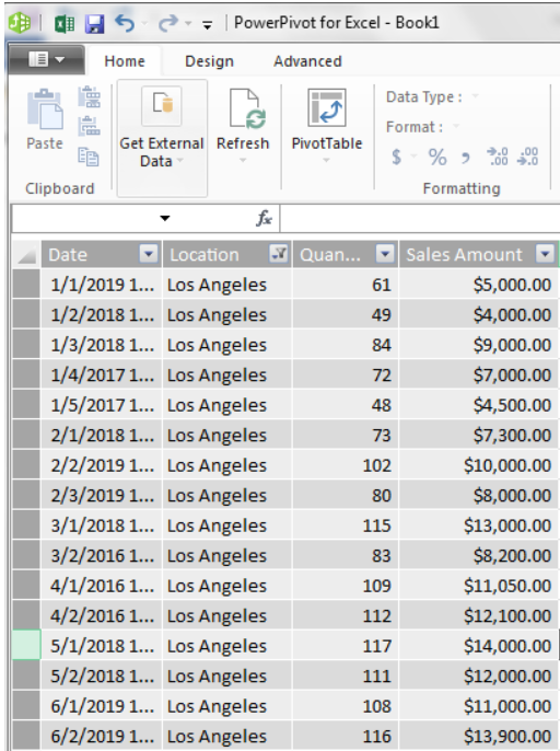 Figure 12- LA Sales
- We will follow the same process and get Las Vegas Sales into Power Pivot
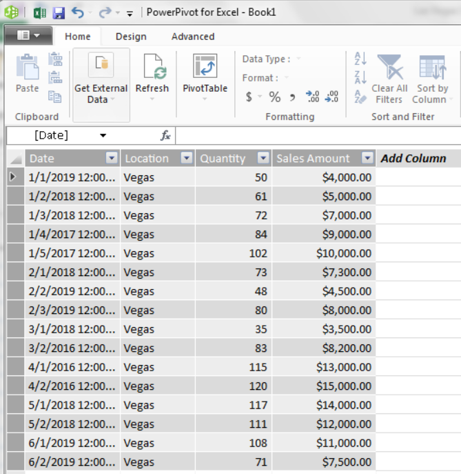 Figure 13- Las Vegas Sales
Creating the Pivot Table
- We will click on anywhere on the table
- We will click on Pivot Table and click on create pivot table
 Figure 14- Creating Pivot Table
- We will click on OK
- We will select and drag the fields to where we want them
 Figure 15- Created Pivot Table
Instant Connection to an Expert through our Excelchat Service
Most of the time, the problem you will need to solve will be more complex than a simple application of a formula or function. If you want to save hours of research and frustration, try our live Excelchat service! Our Excel Experts are available 24/7 to answer any Excel question you may have. We guarantee a connection within 30 seconds and a customized solution within 20 minutes.


Leave a Comment