

Excel uses the default format “General” for values in a cell. This could lead to poor presentation of data especially in a pivot table where we usually deal with massive amount of data in different formats.
Below is an example of a pivot table showing three different number formats: Number with 1000 separator (,), Currency in dollars ($) and Percentage.
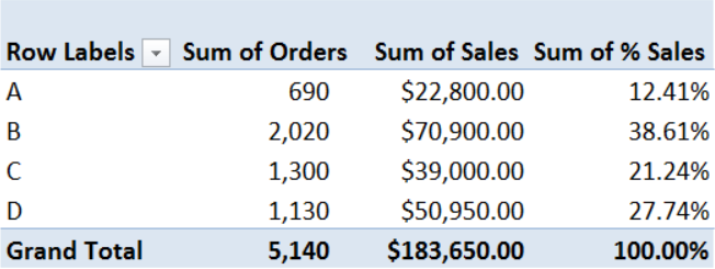 Figure 1. Sample pivot table with different formats per field
Setting up the Data
Here we have a table of product orders and sales from January to February, with corresponding %sales.
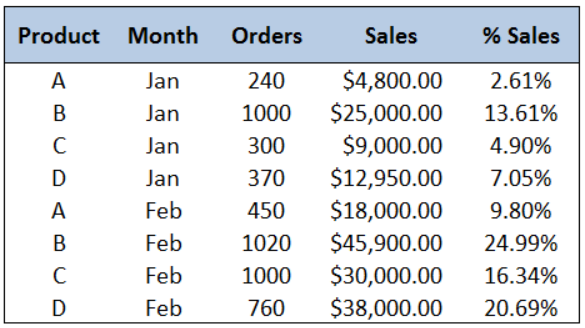 Figure 2. Data for formatting values of numbers in a pivot table
Insert a Pivot Table
Step 1. Select the range of cells that we want to analyze through a pivot table. In this case, we select cells B2:F10.
Step 2. Click the Insert tab, then Pivot Table. This will launch the Create PivotTable dialog box.
 Figure 3. Inserting a Pivot Table
Step 3. In the Create PivotTable dialog box, tick Existing Worksheet. Click the bar for Location and then click cell H2. This will position the pivot table in the existing worksheet, at cell H2.
 Figure 4. Inserting a pivot table in an existing worksheet
Step 4. In the PivotTable Field List, tick Product and Orders. This will show the Sum of Orders for each product from A to D.
 Figure 5. Selecting the fields for values to show in a pivot table
Formatting the Values of Numbers
We have now created a pivot table. We want to change the format for Sum of Orders,which is currently in the default format General.
 Figure 6. Showing the default format for Excel : “General”
There are two ways to format values of numbers.
Method 1. Using Ctrl + 1
Method 2. Using the Value Field Settings
Example 1:
We want to present the Sum of Orders in Number form, with commas for 1000 separator, and no decimal places.
Using Ctrl + 1 Method
Step 1. Select the cells we want to format. In this case, we select I3:I7.
Step 2. Press Ctrl + 1 to launch the Format Cells dialog box.
Step 3. Select the Number Category, then set the decimal places to zero “0”. Tick the Use 1000 separator (,).
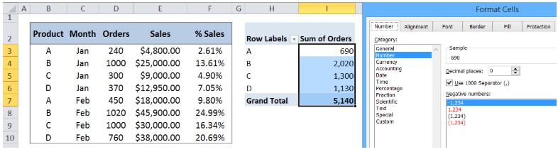 Figure 7. Formatting the values of numbers using Ctrl + 1
We have now changed the format for the Sum of Orders from General to Number.
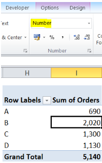 Figure 8. Output: Changing the format of values from “General” to “Number”
Example 2:
We want to add the value Sum of Sales in our pivot table and present it in currency form, with two decimal places.
Method Using the Value Field Settings
Step 1. Tick Sales in the PivotTable Field List. This will add the Sum of Sales in our pivot table.
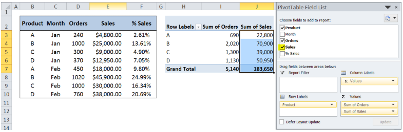 Figure 9. Adding the field Sum of Sales to our pivot table
Step 2. Select the cells that contain the values we want to format (J3:J7), and in the lower right portion of the PivotTable Field List, under Values, click Sum of Sales.
Step 3. Select Value Field Settings.
 Figure 10. Formatting the values of numbers using the “Value Field Settings”
Step 4. In the Value Field Settings dialog box, click Number Format.
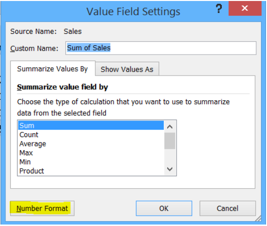 Figure 11. Select “Number Format” in “Value Field Settings”
Step 5. Select the format for Currency, set to 2 decimal places, with the symbol for dollar sign $ English (US).
We have now changed the format for the Sum of Sales in our pivot table.
 Figure 12. Output: Changing the format of values to currency
Let us try adding one more field, %sales.
Example 3:
Step 1. Click any value in the pivot table to show the PivotTable Field List.
Step 2. Select the field %Sales to add the Sum of %Sales to our pivot table.
 Figure 13. Adding more values to our pivot table
Step 3. Select cells K3:K7.
Step 4. Press Ctrl + 1 since it is faster to format the values this way.
Step 5. Select Percentage and set to 2 decimal places.
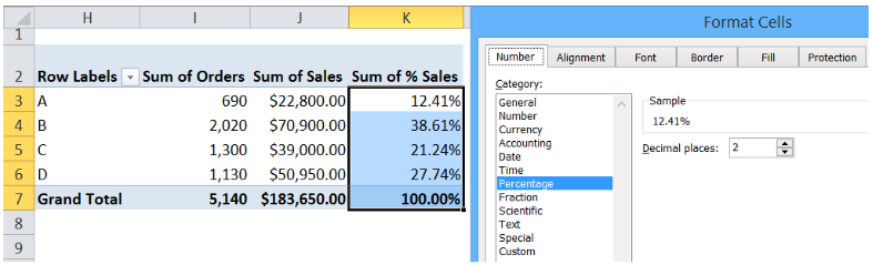 Figure 14. Formatting the values to show percentage
 Figure 15. Final result: Pivot table fields in three different formats
We can now add more values to our pivot table, and change the formatting as we desire.
Most of the time, the problem you will need to solve will be more complex than a simple application of a formula or function. If you want to save hours of research and frustration, try our live Excelchat service! Our Excel Experts are available 24/7 to answer any Excel question you may have. We guarantee a connection within 30 seconds and a customized solution within 20 minutes.


Leave a Comment