

We can use the filters in our PivotTable to retrieve values that we are interested in. For instance, we can retrieve values between a certain number and another. The steps below will walk through the process.
 Figure 1- How to Filter Large Amounts of Data in a Pivot Table
Setting up the Data
- We will use the created pivot table in figure 2 to illustrate how the filter tool works for Pivot Tables.
 Figure 2- Setting up the Data
Value Filters
With the data in our Pivot table, we can use the value filter to check all client expenditure for those lesser than a particular amount. If we want to know the client(s) that spent less than 10,000 at once, we will do the following:
- We will click on the drop-down arrow of Row Labels
- We will click on value filters
- We will select Greater Than or Equal To
 Figure 3- Using Value Filters
- We will insert the amount (10000) into the dialog box and click OK
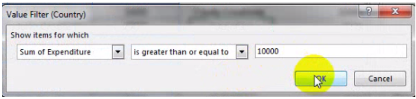 Figure 4- Value Filter (Country) dialog box
 Figure 5- Clients Whose Expenditure is Greater than or Equal to 10,000
- When using filters, it is important to clear the filters after using them, else, they will apply to our next selection or use of the filter
- In figure 6, after deselecting France, the previous filter of values Greater than or Equal To 10000 will still be applied to the result
- We must use “Clear filter from Country” above Label filters in figure 6 if we do not want values Greater than or Equal To 10000 to apply
![]() Figure 6- Clear filters
Figure 6- Clear filters
Top 2 Countries By Sum of Expenditure
- We can use the value filters to find the Top 2 Countries by Sum of Expenditure.
- We will clear all current filters and place our cursor on any country, e.g. Argentina
- We will click on Row Labels, Value filters, and then, Top 10
- We will insert the fields in figure 7 and press OK
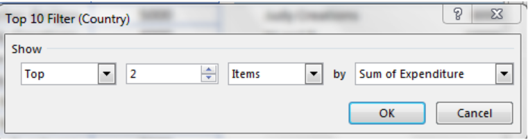 Figure 7- Filter by Country based on Sum of Expenditure
 Figure 8- Top 2 Countries By Sum of Expenditure
- We must note that if we place our cursor on any client, the result will return as Top 2 Client by Sum of Expenditure
Label filters
- We can use the Label filters to find values that contain certain text and several other parameters.
- If we want to find countries that begin with F in our Pivot table, with our cursor on any country or on Rows Labels, we will click on Row Labels, Label filters and Begins with
 Figure 9- Using Label Filters
- We will enter “F” into the dialog box. This isn’t case sensitive
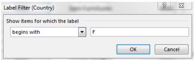 Figure 10- Label filter Dialog box
- We will click OK
 Figure 11- Values that begin with “F”
Instant Connection to an Expert through our Excelchat Service
Most of the time, the problem you will need to solve will be more complex than a simple application of a formula or function. If you want to save hours of research and frustration, try our live Excelchat service! Our Excel Experts are available 24/7 to answer any Excel question you may have. We guarantee a connection within 30 seconds and a customized solution within 20 minutes.


Leave a Comment