

What is a Pivot Table?
A Pivot Table is a table that we can use to analyze, summarize, and calculate data that enables us to visualize trends, comparisons, and patterns in our data in a condensed manner. We can use a Pivot Table to organize a large amount of data in Microsoft Excel.
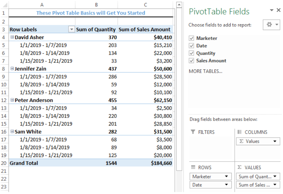 Figure 1: How to Create a Pivot Table
What can we do with a Pivot Table?
- We can set up a Pivot Table in less than a minute
- We can format our Pivot Table as we like it
- We can add data to our Pivot Table by refreshing
- We can set up filters in the Pivot table to have access to only the values we want, etc.
How to Create a Pivot Table
- We will use the data below to create a Pivot Table
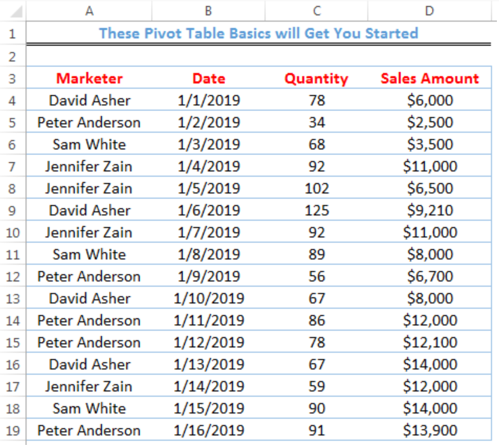 Figure 2: Setting up the Data
Creating a Data Table
Before we create the Pivot Table, we will put the values in figure 2 into a table.
- We will click on anywhere on the data, click on the Insert tab, and click on Table as shown in figure 3
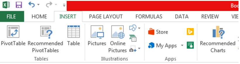 Figure 3- Putting the data in a Table
- We will click on OK on the dialog box that appears once the table range is selected
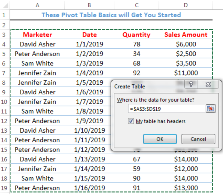 Figure 4- Create Table Dialog Box
 Figure 5- Created Table
- We will click on the box below Table Name under File in Figure 5 and name the Table as Sales_Data
- We will press enter after inserting the name
- We can add some designs to the table by going to Design and make a choice
 Figure 6- Selecting a Table design
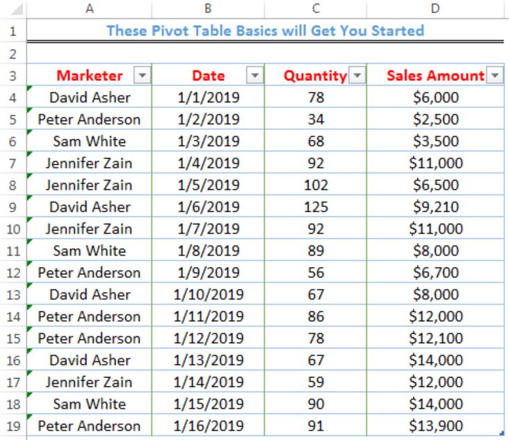 Figure 7- Applying Table Design
- The drop-down arrows on Row 1 of the Table can be used to filter data
- Now, we will create a Pivot Table with the Data
Creating the Pivot Table
- We will click on anywhere on the table
- We will click on the Insert tab and click on Pivot Table as shown in figure 3
 Figure 8- Create Pivot Table Dialog Box
- We will click on New worksheet
- We will click OK
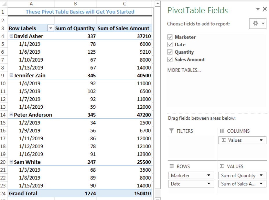 Figure 9- Created Pivot Table and Selected Pivot Table Fields
- We can drag any of the fields to the “Drag fields between areas below section” to adjust how our table will look
Formatting the Pivot Table
We can format our Pivot Table by refreshing our Pivot Table whenever we add new data to the data table, applying number formatting (e.g. with Currency), and using the filter options
Refreshing the Pivot Table
We can expand the Range of the Table by taking our cursor to the edge as shown in figure 10 and drag down
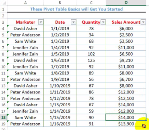 Figure 10a: Expanding the Range of the Data Table
 Figure 10b: Expanding the Range of the Data Table
- We will insert new values into the empty cells
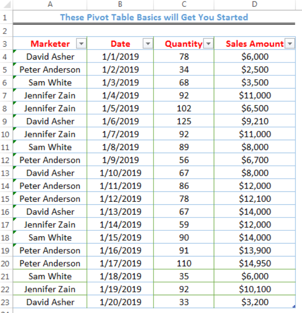 Figure 11: Values inserted into the Expanded Range of the Data Table
- Our Pivot Table doesn’t automatically update as we add these values
- We will click on the Pivot Table, right-click, and click on Refresh
 Figure 12: Refreshed Pivot Table with New Data
- We have condensed the details of Sam White so that we will have a full view of the Pivot table. Double-clicking on Sam White will result in the details displaying
Number Formatting
- We can format the Sum of Sales Amount in figure 12 to have a particular currency like the United States Dollar ($)
- We will click on any cell of the Sum of Sales Amount Column
- We will right-click and click on Number format
 Figure 13: Format Cells Dialog Box
- We will click on Currency and set the decimal places to 0. We will also set the symbol as $
- We will click OK
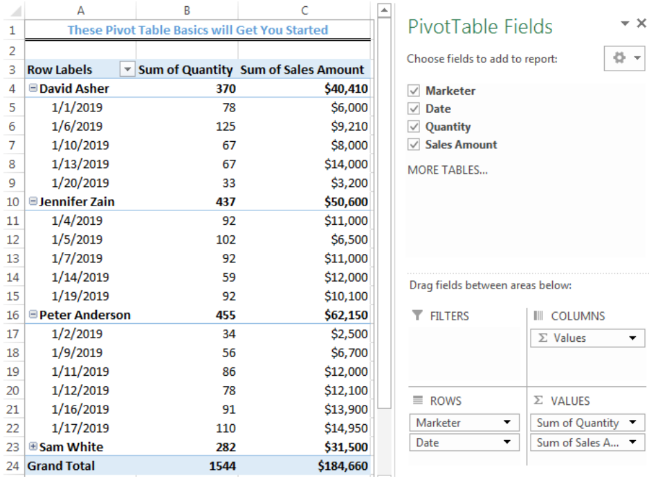 Figure 14: Formatted Cells with Currency ($)
Grouping Pivot Table Data
We can group the Data in the Pivot Table to know Sum of Sales Amount and the Sum of Quantity within every 7 days.
- We will click on any of the dates
- We will right-click and click on group
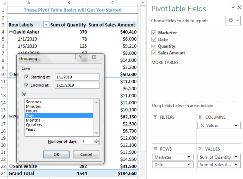 Figure 15- Grouping Dialog Box
- We will click on Days and set number of days to 7
- We will click OK
 Figure 16- Pivot Table grouped by Days
Instant Connection to an Expert through our Excelchat Service
Most of the time, the problem you will need to solve will be more complex than a simple application of a formula or function. If you want to save hours of research and frustration, try our live Excelchat service! Our Excel Experts are available 24/7 to answer any Excel question you may have. We guarantee a connection within 30 seconds and a customized solution within 20 minutes.


Leave a Comment