How to Update a Pivot Table in Excel

In Excel, when we add data or make changes in the source data set, the Pivot Table does not pick up these changes automatically in the data set. We need to refresh the Pivot table manually as standard functionality in Excel to update the Pivot table results with these changes in source data. In this article, we will learn how to refresh the Pivot table in Excel manually to update Pivot Table results.

1. Changing data in source data set

When we change any text or number in existing source data range, then this change is not automatically captured in the Pivot Table, so we need to refresh the Pivot table manually.

In Excel, while inserting a Pivot table, we need to select the source data range, like Sheet1!$A$1:$E$46 to include this dataset as source data for Pivot table. So, if we change or edit any text or numbers in this source data range Sheet1!$A$1:$E$46, then we need to refresh Pivot table to update results.

To refresh a Pivot table after changing data in a source data set, we need to follow the following steps;

Go to the Pivot Table worksheet and click any cell inside the Pivot table
Go to Pivot Table tools > On Options /Analyze Tab > In Data group, click on Refresh. Or Right-click inside the Pivot table, and click on Refresh
Alternately, press ALT+F5 short keys to refresh Pivot Table

2.Adding or deleting data in source data

When we add or delete data in a source data by adding or deleting rows and columns, then we need to refresh the Pivot table. In this way the size of source data changes, but this change does not take effect in Pivot table automatically. So, we need to change Data Source in Pivot table to update Pivot table results. Source data can be changed in two ways;

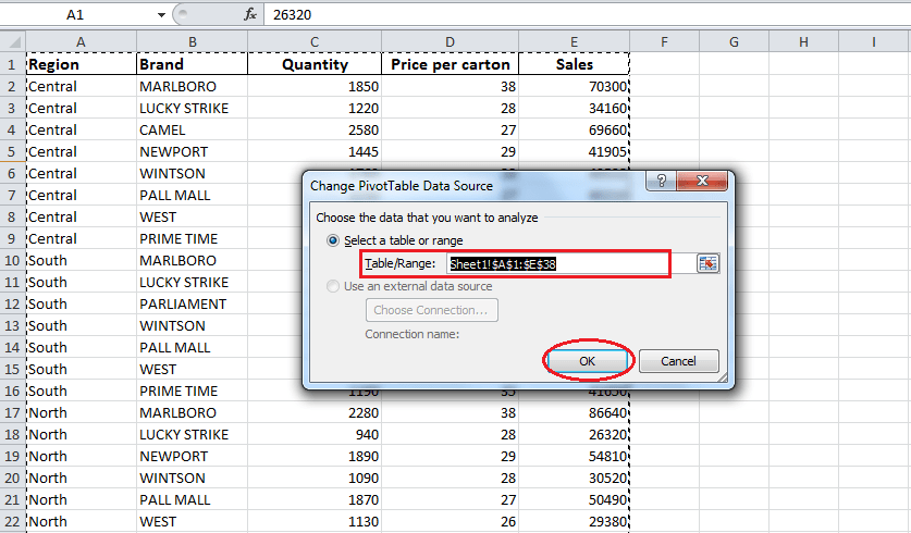
Manually Change Data Source: After adding or deleting data from source data, we can manually change data source in a Pivot table to refresh the Pivot table. In order to do that, click any cell inside the pivot table > Go to Pivot Table tools > On Options /Analyze Tab > In Data group, click on Change Data Source

A new dialog box appears. In Table/Range section, a select new range of source data or table or Excel automatically selects the available range in the source data sheet, and press OK to refresh the Pivot table.
Dynamically Change Data Source. Another way to change the data source is to format your source data as a Table before inserting the Pivot table. In this way, your data source will be updated automatically when you add or delete rows and columns in the source data. You do not need to change the data source manually, but you still have to refresh the Pivot table manually. In order to do that;
Click any cell in source data > Go to Insert tab, Click on Table from Tables section. This way your source data will be formatted as Table, and now you insert the Pivot table.

A “Create Table” dialog box appears it will select available source data to format as Table and press OK button.

After formatting source data as a Table, you can insert a Pivot table. When you add or delete data in the source data sheet, your source data automatically updates in the Pivot Table, but you only need to manually refresh the Pivot table as discussed earlier.

3.Refresh Pivot Table On File Open

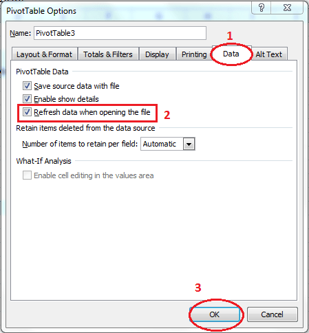
You can automatically refresh the Pivot table when you open the file in Excel. After updating the source data, and when you open this file next time, the Pivot Table will be updated automatically. To do that, you need to update the Pivot table options. Please follow these steps.

Click any cell inside Pivot table, click Options/Analyze tab, click Options > Options in the Pivot table group
The pivot table options dialog box appears, click Data tab and check Refresh data when opening the file and press OK

Still need some help with Excel formatting or have other questions about Excel? Connect with a live Excel expert here for some 1 on 1 help. Your first session is always free.