

We can use a PivotTable to analyze, summarize and calculate data that enables us to visualize trends, comparisons, and patterns in our data. The steps below will walk through the process of Inserting a Pivot Table in Excel.
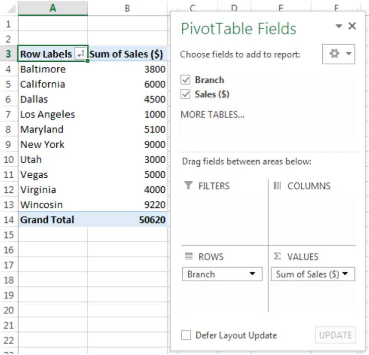 Figure 1- How to Insert a Pivot Table in Excel
Setting up the Data
- We will create a Pivot Table with the Data in figure 2.
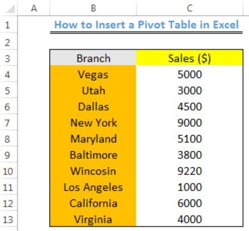 Figure 2 – Setting up the Data
Creating the Pivot Table
- We will select the range (B3:C13) of the table
- We will click on the Insert tab and click on Pivot Table
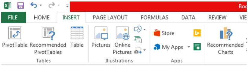 Figure 3- Clicking on Pivot Table
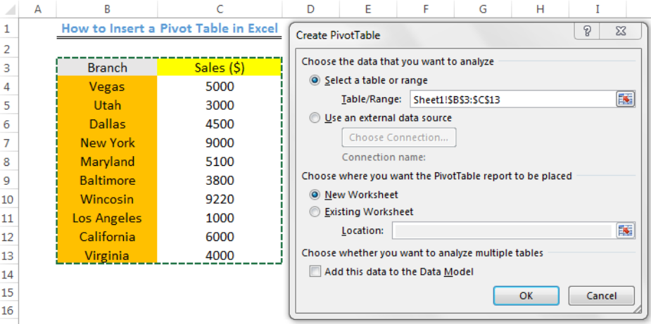 Figure 4- Creating the Pivot Table
- We will click on OK to create the Pivot Table in a New Worksheet
- We will select the fields we want to add to the Pivot Table
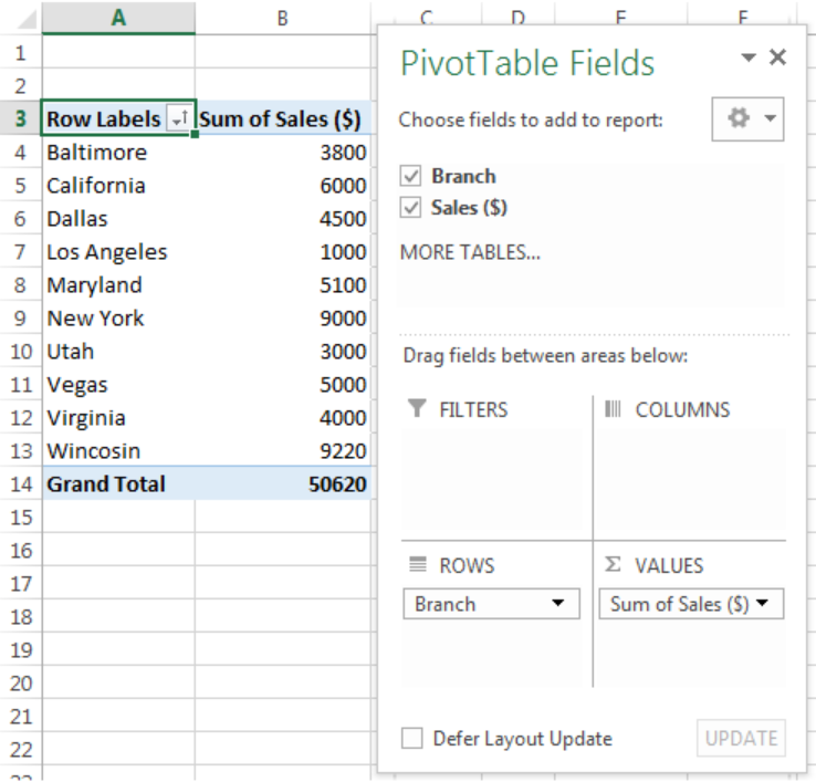 Figure 5- Created Pivot Table
- We can also add a little change to the Pivot Table by dragging the Sales ($) in the Choose fields to add to report to the COLUMNS beside FILTERS
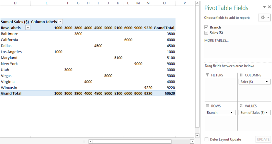 Figure 6- Pivot Table
Note
- Under “Choose where you want the PivotTable report to be placed”, we can specify the location where we want the worksheet to be placed. Assuming we select “Existing Worksheet”, a valid location will be an unoccupied cell in the existing worksheet, e.g. Sheet1!$D$3
Instant Connection to an Expert through our Excelchat Service
Most of the time, the problem you will need to solve will be more complex than a simple application of a formula or function. If you want to save hours of research and frustration, try our live Excelchat service! Our Excel Experts are available 24/7 to answer any Excel question you may have. We guarantee a connection within 30 seconds and a customized solution within 20 minutes.


Leave a Comment