

We can use a PivotTable to GROUP A SET OF DATA like dates, months, years, quarters, etc. This enables us to analyze, summarize, calculate, and visualize trends, comparisons, and patterns in our data. The steps below will walk through the process of Grouping Pivot Table Data.
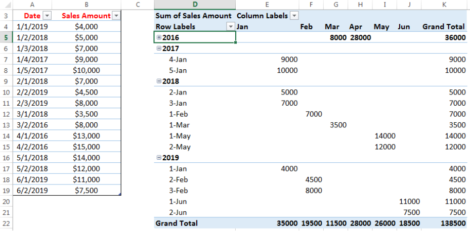 Figure 1- How to Group Pivot Table Data
Setting up the Data
- We will open a New excel sheet
- We will input dates when sales were made in Column A and the corresponding Sales Amount in Column B
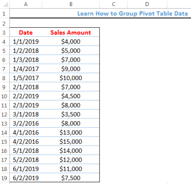 Figure 2- Setting up the Data
- We will click on anywhere on the table, click on the Insert tab, and click on Table as shown in figure 3
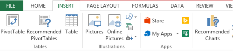 Figure 3- Putting the data in a Table
- We will click on OK on the dialog box that appears
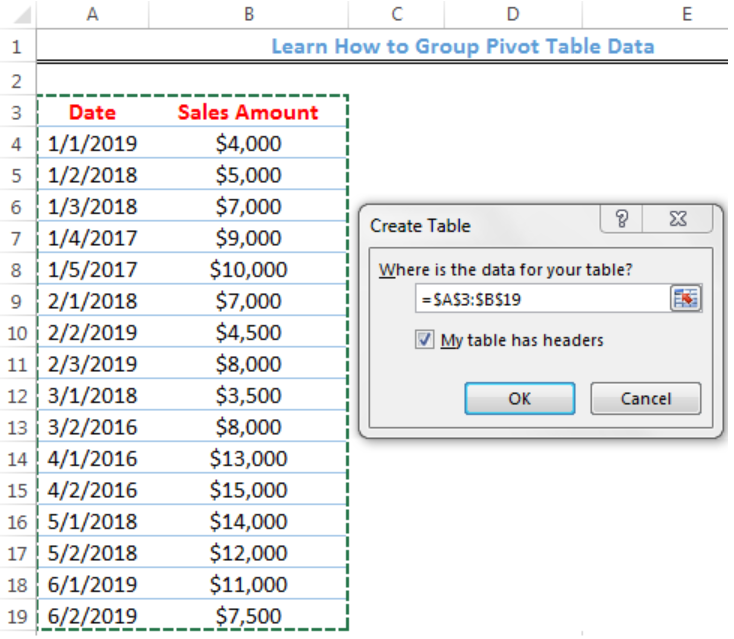 Figure 4- Create Table Dialog Box
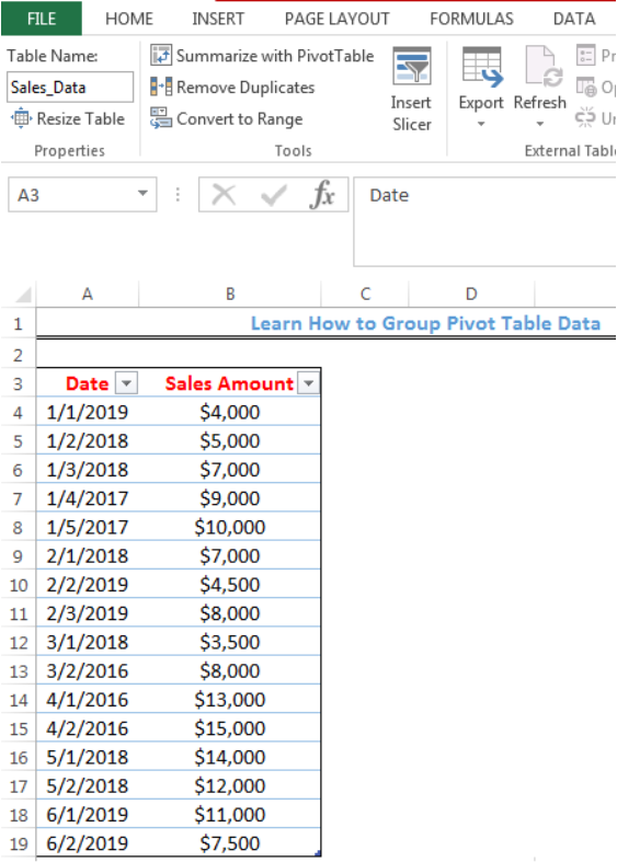 Figure 5- Created Table
- We will click on the box below Table Name under File in Figure 5 and name the Table as Sales_Data
- We will press enter after inserting the name
- Now, we will create a Pivot Table with the Data
Creating the Pivot Table
- We will click on anywhere on the table
- We will click on the Insert tab and click on Pivot Table as shown in figure 3
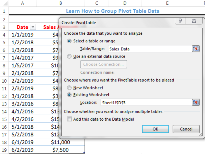 Figure 6- Creating the Pivot Table
- We will click on existing worksheet and specify the Location where the Pivot table will start from (Sheet1!$D$3)
- We will click on OK
- We will select the fields we want to add to the Pivot Table (Dates and Sales Amount)
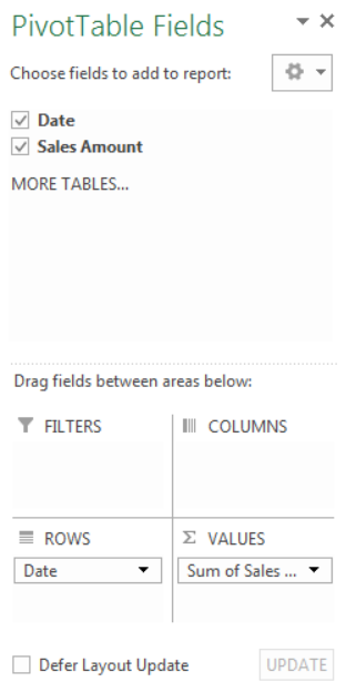 Figure 7- Selecting Pivot Table Fields
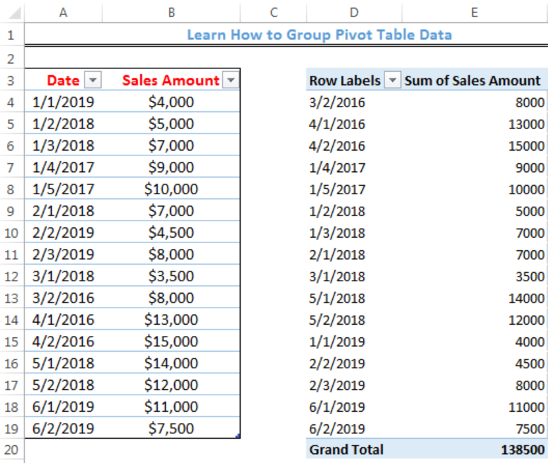 Figure 8- Pivot Table
Grouping the Pivot Table Data by Year
- We will click on any date within the Pivot Table
- We will right-click and click on GROUP
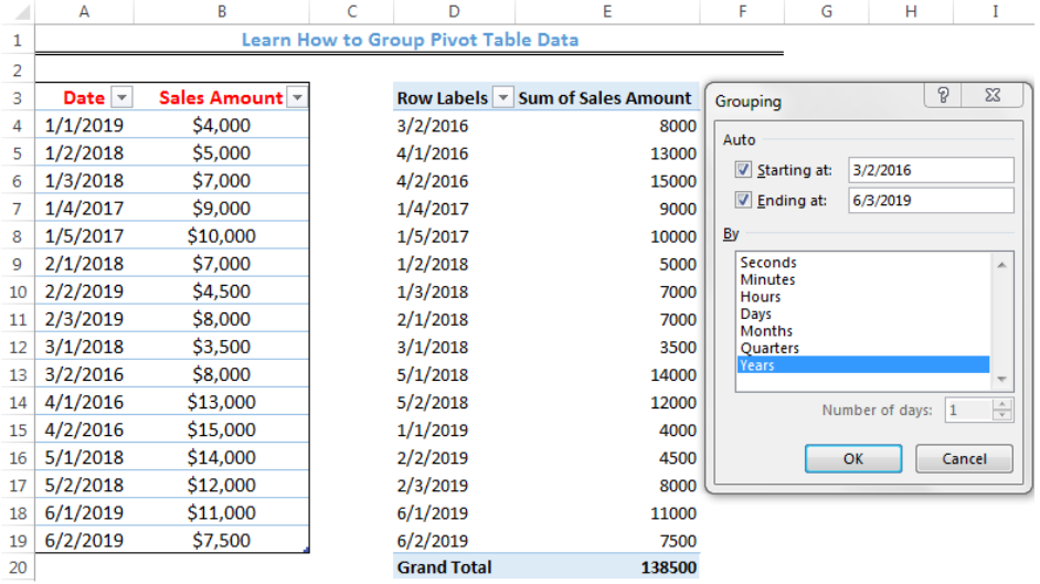 Figure 9- Grouping Dialog box
- We will click OK
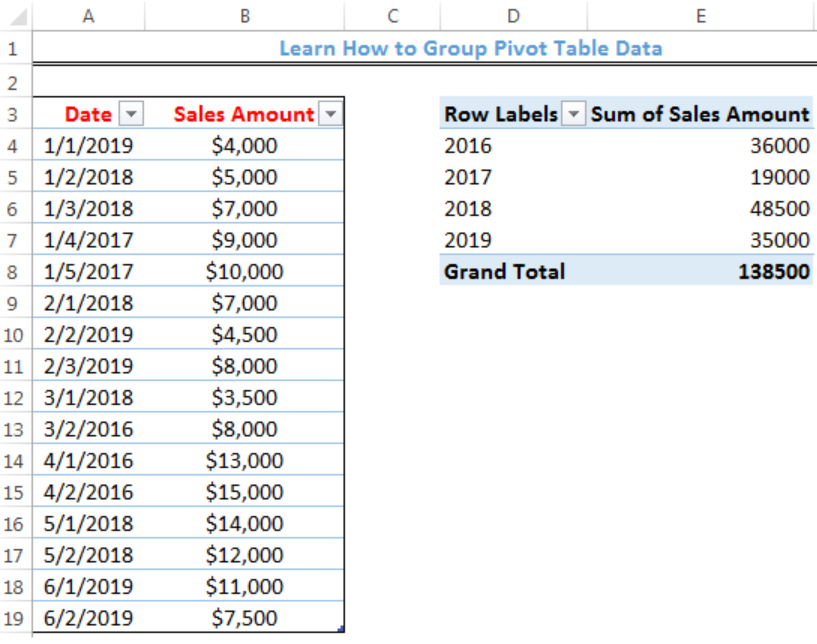 Figure 10- Pivot Table Grouped by Year
Grouping the Pivot Table Data by Days
In the same way, AS DESCRIBED FOR GROUPING BY YEAR, we can select days as shown in figure 10, specify the number of days, and click OK.
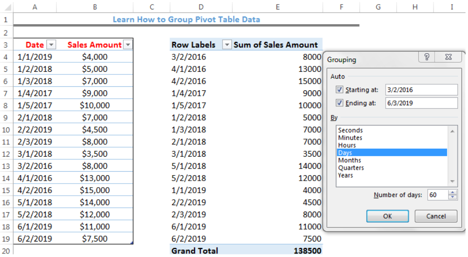 Figure 11- Grouping Dialog box
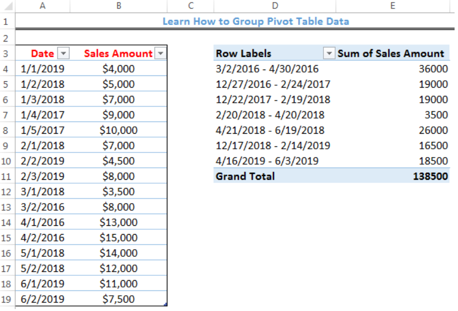 Figure 12- Pivot Table Grouped by Days
- The same procedure can be followed to group pivot table data by months and quarters.
Grouping the Pivot Table Data by Days, Months, and Year
- We can group our Pivot Table by clicking on the three options; Days, Months, and Year on the grouping dialog box
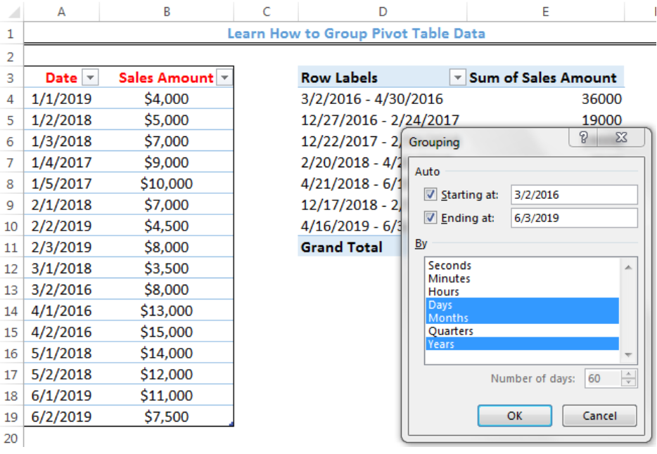 Figure 13- Grouping the Pivot Table Data by Days, Months, and Year
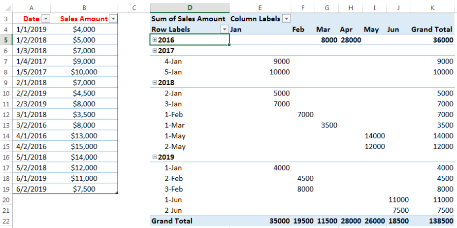 Figure 14- Grouped Pivot Table Data by Days, Months, and Year
- We should note that we have clicked on the dash (–) sign for 2016 to hide the details for us to have a full view of the Pivot table. Also, the arrangement of the Columns and rows is by dragging the Pivot Table Fields to the locations as shown in Figure 15
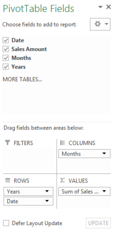 Figure 15: Pivot Table fields for Grouping by Days, Months, and Year
Note
- Double-clicking on any of the Row labels will drop-down or hide the details for that year
Instant Connection to an Expert through our Excelchat Service
Most of the time, the problem you will need to solve will be more complex than a simple application of a formula or function. If you want to save hours of research and frustration, try our live Excelchat service! Our Excel Experts are available 24/7 to answer any Excel question you may have. We guarantee a connection within 30 seconds and a customized solution within 20 minutes.


Leave a Comment