

We can use the GETPIVOTDATA function to get the Grand total in our pivot table. The steps below will walk through the process.
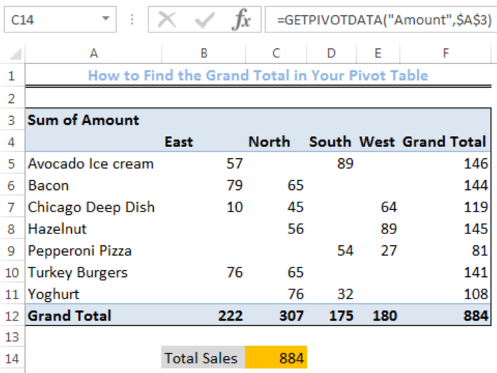 Figure 1 – Using GETPIVOTDATA to get pivot table grand total
General formula
=GETPIVOTDATA("field name",pivot_ref)
Formula
=GETPIVOTDATA("Amount",$A$3)
Setting up the Data
- We will set up our data in an array of rows and columns as shown below
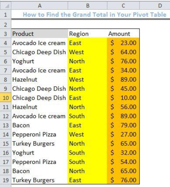 Figure 2 – Setting up the Data
- We will create a simple pivot table from our data. With it, we will apply our function to arrive at the grand total
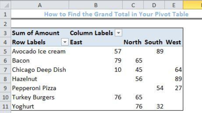 Figure 3 – Creating a simple pivot table
Pivot Table Grand Total
- We will click on any cell in the worksheet outside our Pivot table
- In this cell, we will enter the formula below
=GETPIVOTDATA("Amount",$B$4) - We will press the enter key
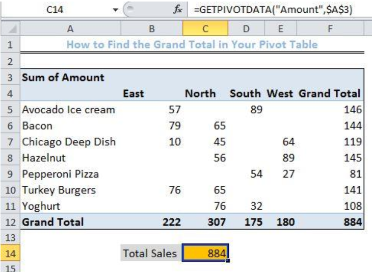 Figure 4 – How to get the pivot table grand total
An alternative way to get the pivot table grand total
We can equally use a faster approach to insert our pivot table grand total into the worksheet.
- After we have created the pivot table, we will go to Pivot table Design, Click on Grand Totals and lastly, select “on for Rows and Columns.”
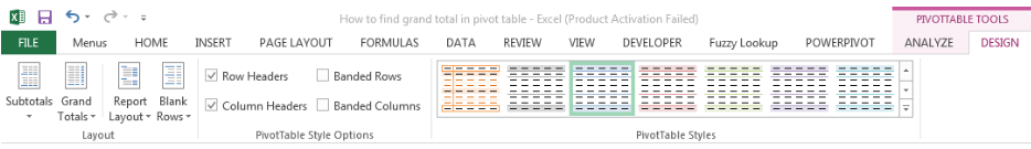 Figure 5- Click on Pivot table design
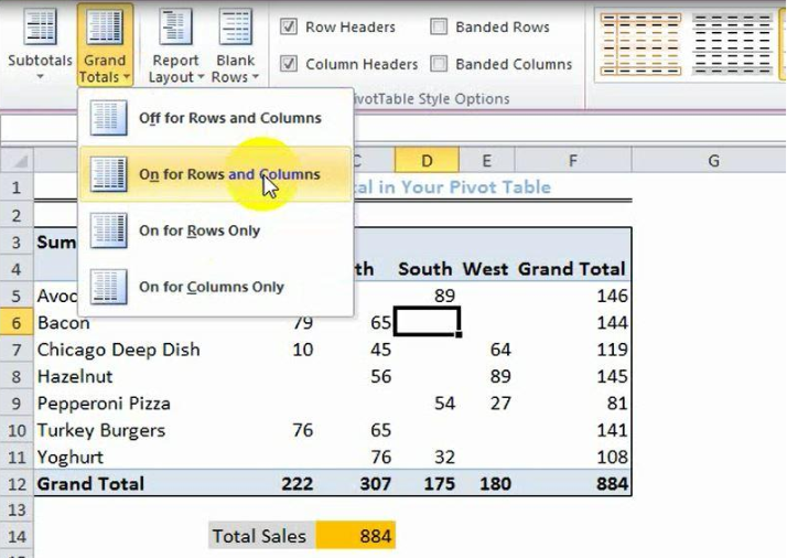 Figure 6 – Alternative option to achieve the pivot table grand total
Note
The GETPIVOTDATA function is dependent on the value field. Therefore whatever we set for the value field (e.g., sum, count, average, etc.) will affect the value of our grand total.
Instant Connection to an Expert through our Excelchat Service
Most of the time, the problem you will need to solve will be more complex than a simple application of a formula or function. If you want to save hours of research and frustration, try our live Excelchat service! Our Excel Experts are available 24/7 to answer any Excel question you may have. We guarantee a connection within 30 seconds and a customized solution within 20 minutes.


Leave a Comment