We may have blank cells in our Pivot table from time to time. In this tutorial, we will explore how we will deal with pivot table blanks.
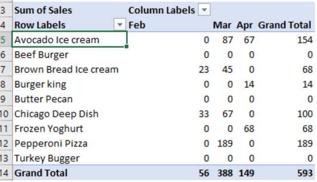 Figure 1 – Showing zero in pivot blank cells
Setting up the Data
- First, we will create our sample worksheet
- Next, Column A, B, and C will contain our Dates, Products, and Sales respectively
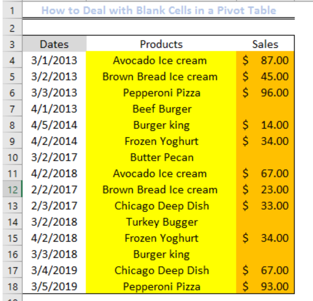 Figure 2 – Setting up our raw data
- Next, we will create our pivot table by clicking on the Insert tab and select Pivot table
 Figure 3- Clicking on Pivot Table
- We will create the Pivot table in a new worksheet
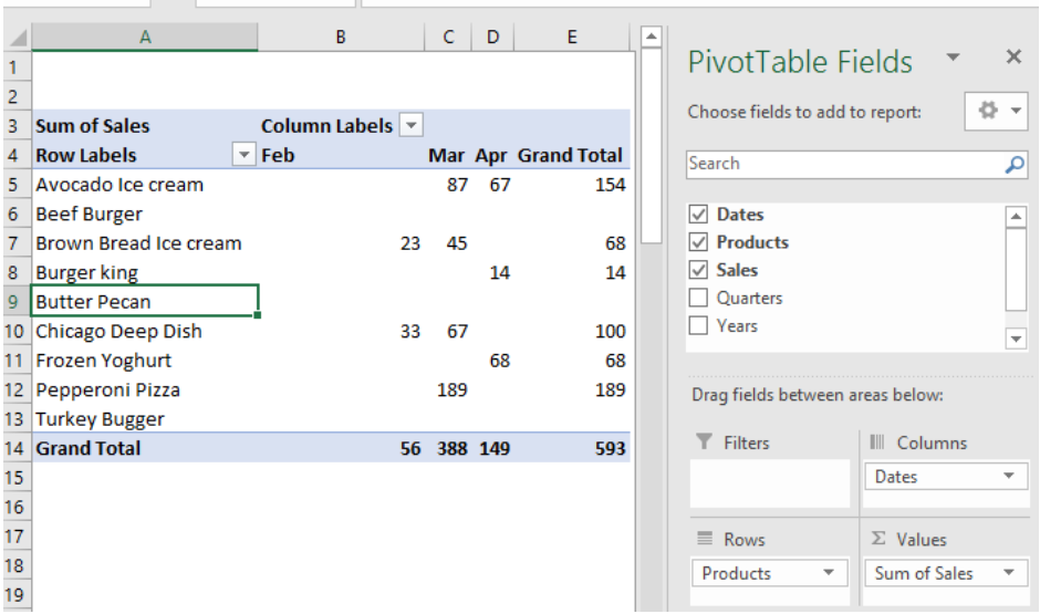 Figure 4 – Setting up our Pivot table
Dealing with pivot table blank cells
- We will right-click anywhere in the pivot table and select PivotTable options
 Figure 5 – Clicking on Pivot table options at the Far left
- In the PivotTable Options dialog box, we will select Layout & Format
- In the format section, we will insert text like TBD in the For empty cells show box
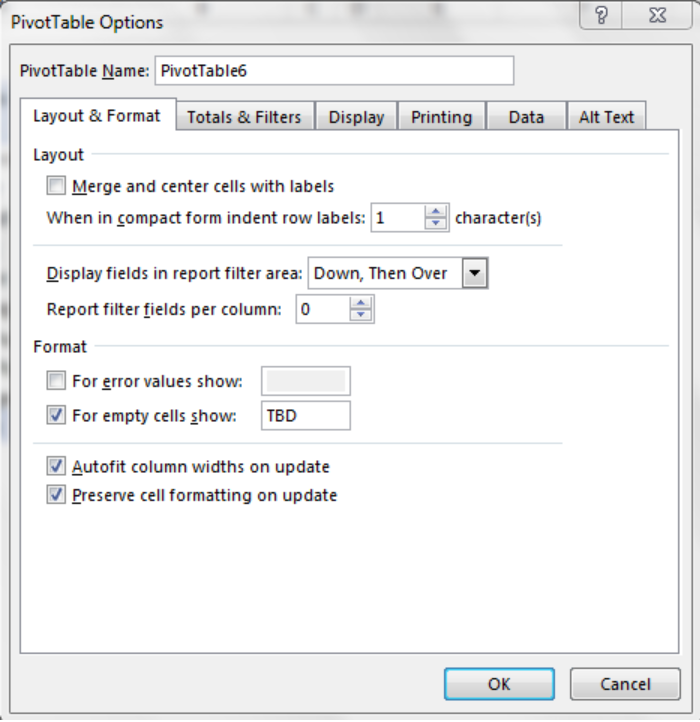 Figure 6 – PivotTable options dialog box
- We will click OK
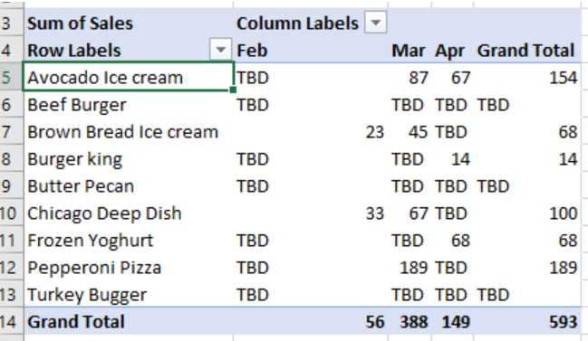 Figure 7 – Setting pivot blank cells to contain text
Showing zero in pivot blank cells
We can alternatively make our blank cells to show zero as well. To do this, right-click anywhere in the pivot table. Select Pivot Table options, then Layout & Format and lastly, unmark For empty cells show option.
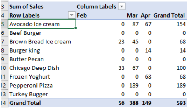 Figure 8 – Showing zero in pivot blank cells
Instant Connection to an Expert through our Excelchat Service
Most of the time, the problem you will need to solve will be more complex than a simple application of a formula or function. If you want to save hours of research and frustration, try our live Excelchat service! Our Excel Experts are available 24/7 to answer any Excel question you may have. We guarantee a connection within 30 seconds and a customized solution within 20 minutes.


Leave a Comment