

We sometimes need to customize our pivot tables and create calculated fields and items. This step by step tutorial will assist all levels of Excel users in calculating pivot table data.
 Figure 1. Final result: How to calculate pivot table data
Setting up Our Data
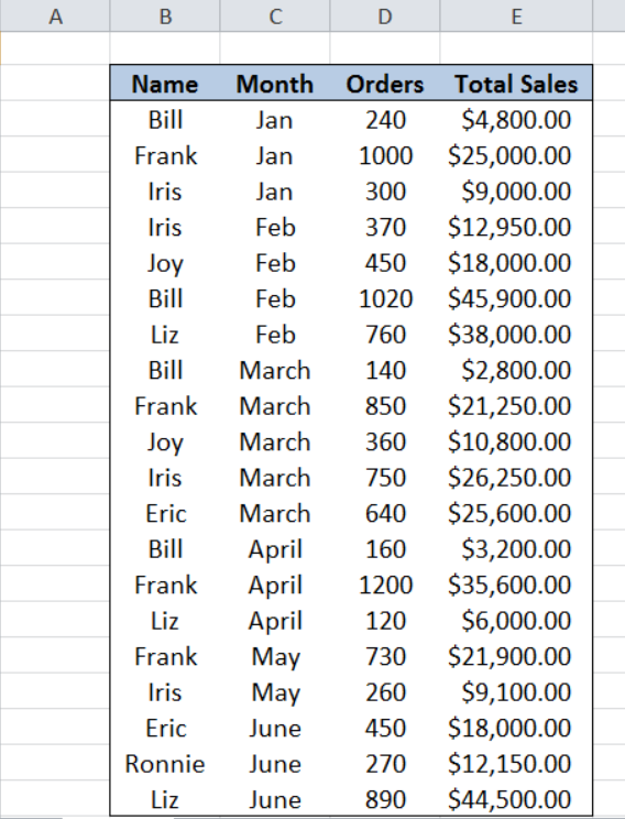 Figure 2. Sample data: How to calculate pivot table data
Our table consists of four columns: Name (column B), Month (column C), Orders (column D) and Sales (column E). First, let us insert a pivot table using our data.
Insert a pivot table
In order to insert a pivot table, we follow these steps:
Step 1. Select the cells of the data we want to use for the pivot table. In this case, select cells B2:E22
Step 2. Click the Insert tab, then select PivotTable
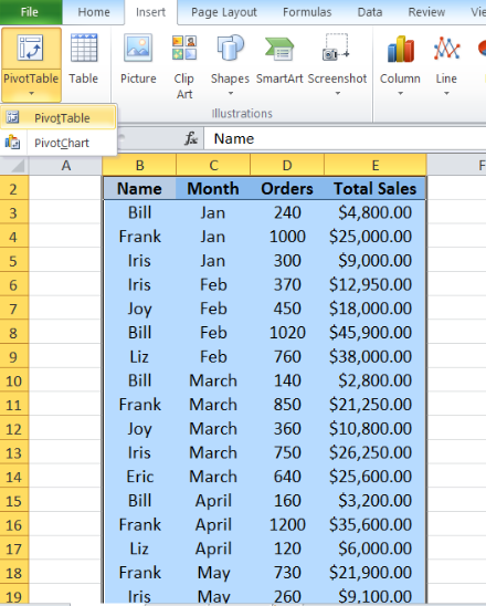 Figure 3. Selecting the data to insert a pivot table
Step 3. In the Create PivotTable dialog box, tick Existing Worksheet. Click the Location bar and then click cell G2.
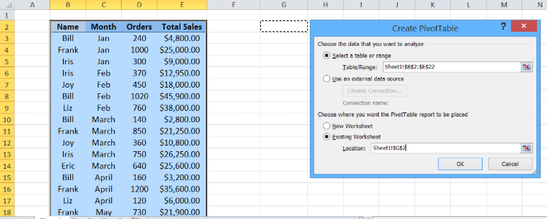 Figure 4. Inserting a pivot table in existing worksheet
Step 4. In the PivotTable Field List, click Name, Month and Total Sales
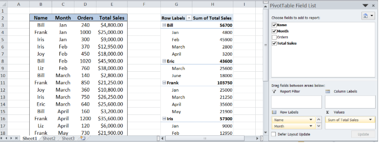 Figure 5. Creating a pivot table with chosen fields
We have now successfully created our pivot table. Note that the total sales per person is categorized by month. We want to improve our pivot table such that
- It shows the sales for the 1st and 2nd quarter, by adding a calculated item
- It shows the commission of each person based on sales, by adding a calculated field
The main difference between calculated item and field is this: we use calculated item when we want to add a formula using data from specific items within a field; we use calculated field when we want to add a formula using data from another field.
Create calculated items for 1st and 2nd quarter
In order to create calculated items showing the sales for 1st quarter and 2nd quarter, we follow these steps:
Step 1. Click any cell under a specific field to enable creation of a calculated item
Step 2. Under the Options tab, click Fields, Items, & Sets, then select Calculated Item
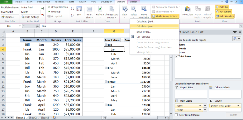 Figure 6. Adding a calculated item
Step 3. In the name bar, enter “1st Quarter”
Step 4. In the formula bar, enter the formula: =Jan+ Feb+ March
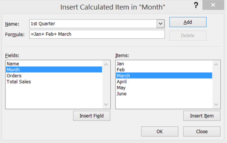 Figure 7. Inserting a new calculated item: 1st Quarter
Step 5. Click Add, then OK.
Step 6. Repeat steps 1 to 5 but this time, enter “2nd Quarter” for the Name and =April+May+June for the Formula.
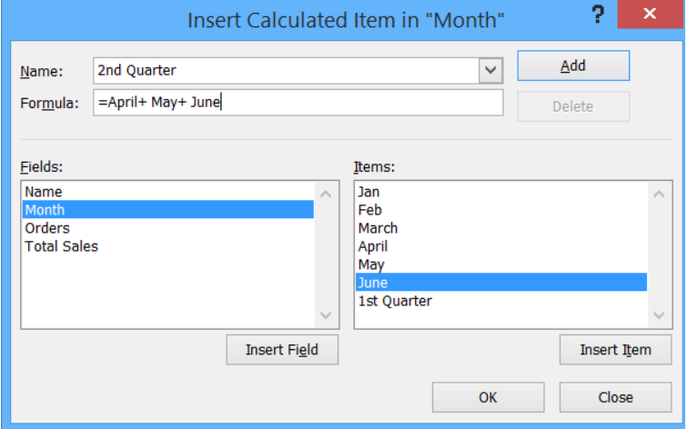 Figure 8. Inserting another calculated item: 2nd Quarter
We have created the two calculated items 1st Quarter and 2nd Quarter.
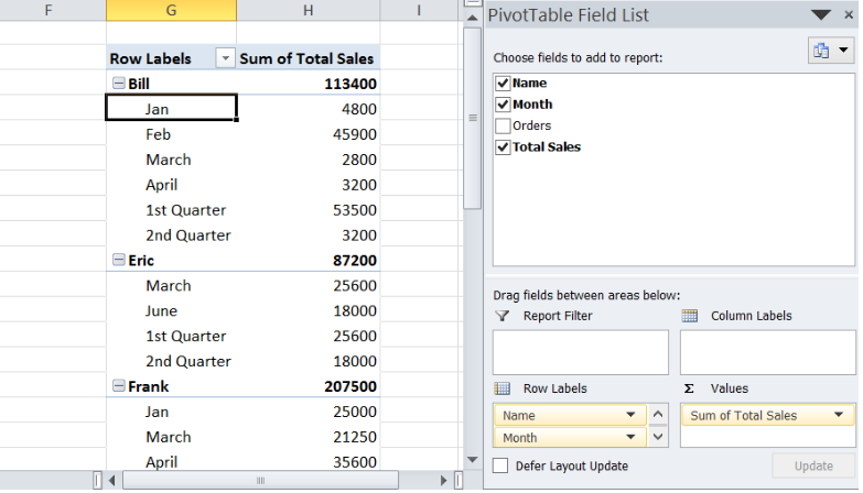 Figure 9. Output: New calculated items added to pivot table
Next we filter the data to show only the 1st and 2nd Quarter.
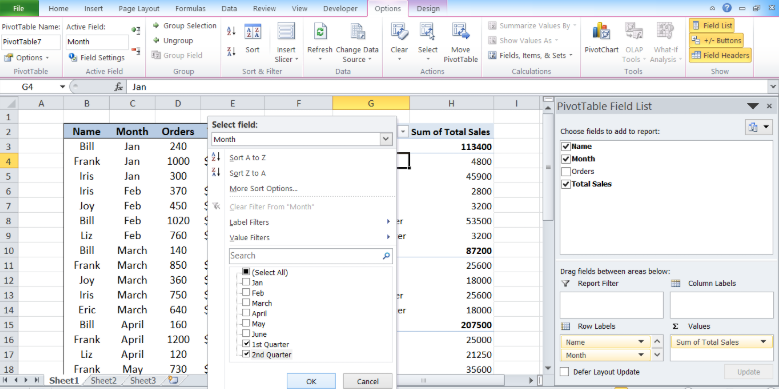 Figure 10. Selecting the items to display in pivot table
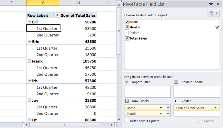 Figure 11. Output: Pivot table showing calculated items
Create calculated field for commission
In order to create a calculated field showing the commission per person, we follow these steps:
Step 1. Click any field name. In this case, we click G2
Step 2. Under the Options tab, click Fields, Items, & Sets, then select Calculated Field
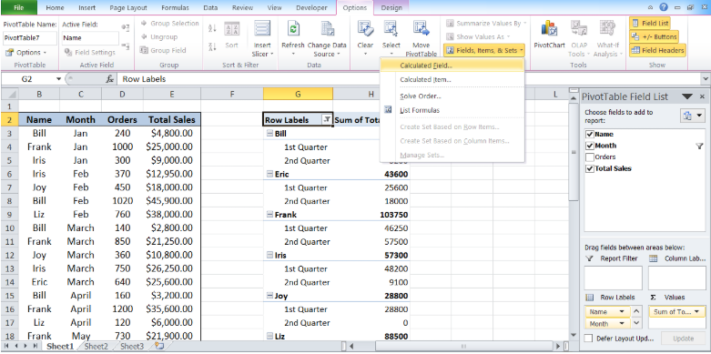 Figure 12. Adding a calculated field
Step 3. In the name bar, enter “Commission”
Step 4. In the formula bar, enter the formula: =’Total Sales’*0.05
Our formula for commission is 5% of the total sales.
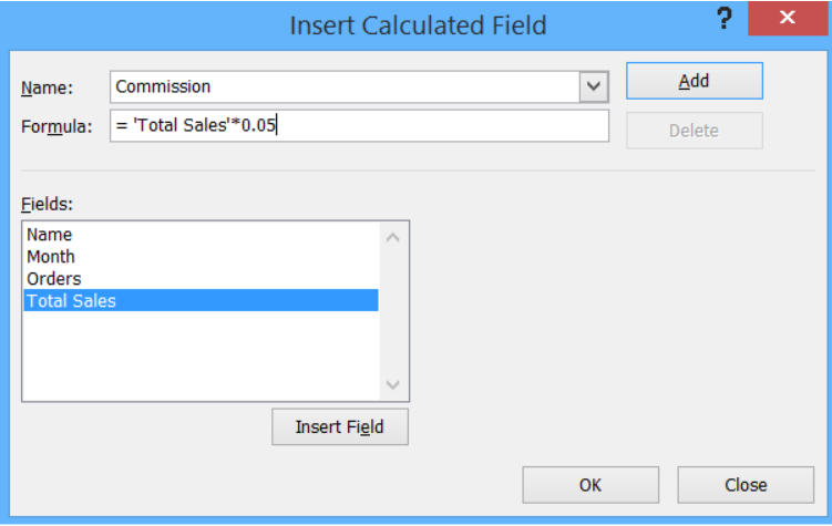 Figure 13. Inserting a new calculated field for Commission
Step 5. Click Add, then OK.
A new calculated field “Commission” has been added under “Total Sales”.
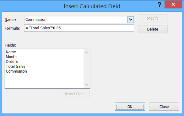 Figure 14. Output: Adding a calculated field “Commission”
Going back to our pivot table, a new field has been added, showing the sum of commission per person.
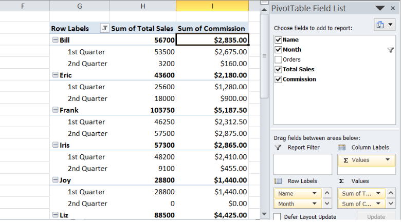 Figure 15. Final result: How to calculate pivot table data
Finally, we have calculated pivot table data by adding both calculated items and calculated field.
Most of the time, the problem you will need to solve will be more complex than a simple application of a formula or function. If you want to save hours of research and frustration, try our live Excelchat service! Our Excel Experts are available 24/7 to answer any Excel question you may have. We guarantee a connection within 30 seconds and a customized solution within 20 minutes.


Leave a Comment