The Procedure for Calculating a Percentage in a Pivot Table

Are you struggling with calculating a percentage in a pivot table? Pivot tables in Excel are excellent tools for analyzing data. They help you to aggregate, summarize, finding insights and presenting a large amount of data in just a few clicks, including calculating a percentage from given data.

You can create and modify pivot tables very quickly. You can create calculated fields in a pivot table that help expand your analysis with more data. Though it has some limitations, calculated fields are a great way to find new insights, such as percentages, from pivot tables.

Calculating percentage in the pivot table

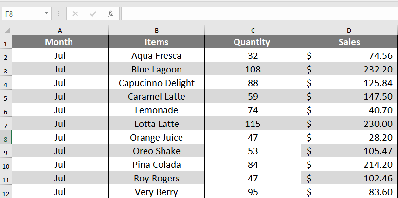
In this example, you have the beverage sales data of eleven items for the 3rd quarter of the year.

Create and format your pivot table

To create the Pivot Table and apply conditional formatting, you need to perform the following steps:

1. Click anywhere in the data.
2. Go to Insert > Recommended PivotTables. Scroll down and select the one that says Sum of Sales by Items and Month.

3. Click OK.

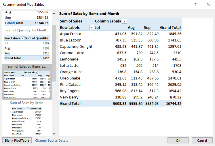
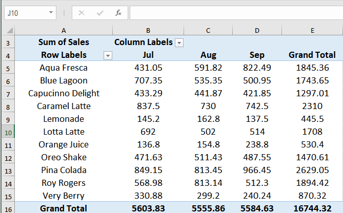
You will have the pivot table with the Sales for the Items for each Month.

To calculate % of Sales for each month, you need to do the following:

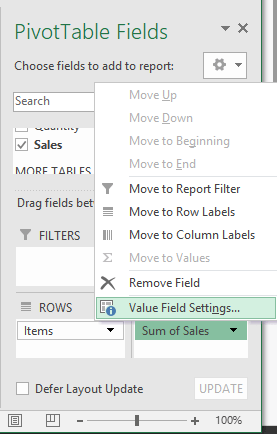
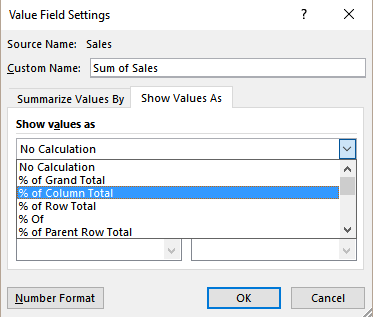
1. Click on pivot builder the entry Sum of Sales and select Value Field Settings.
2. In the Value Field Settings window, on the Show Values As tab, choose % of Column Total.

3. Click OK.

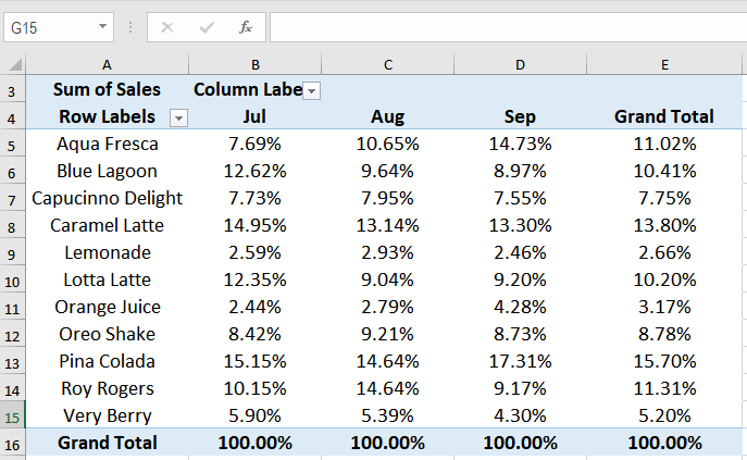
This would show the sales for each item as the percentage of total monthly sales.

Create the calculated field in the pivot table

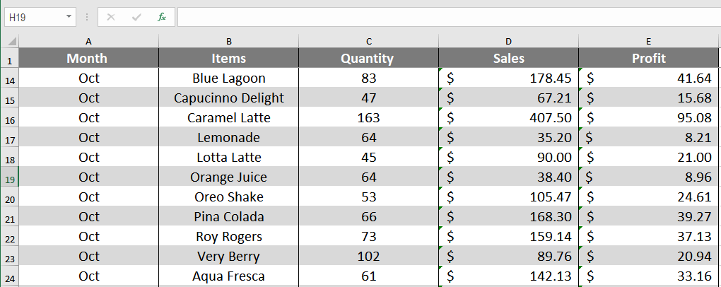
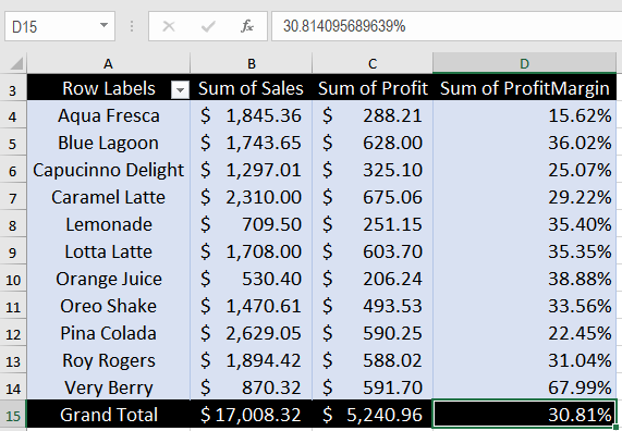
A calculated field is a column generated by the data in the pivot table. For this example, we will use the sales and profit data for the eleven items during the 4^th quarter of the year.

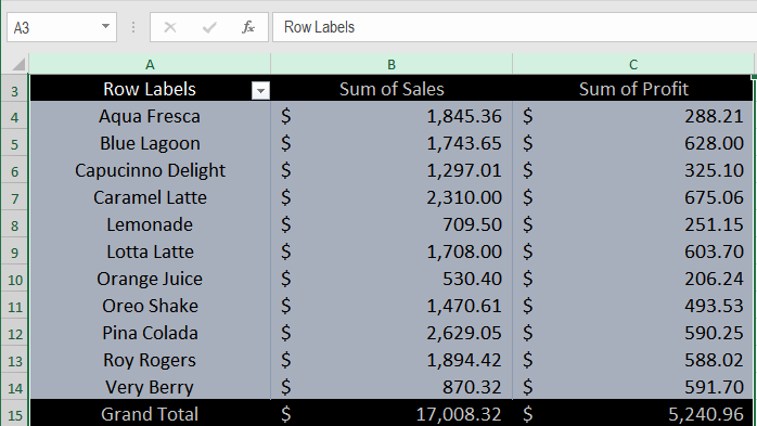
From this, we have the pivot table Sum of Sales and Profits for the Items.

To add the profit margin for each item:

1. Click on any cell in the Pivot Table.
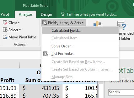
2. Go to (Pivot Table Tools) Analyze > Fields, Items, & Sets > Calculated Field.

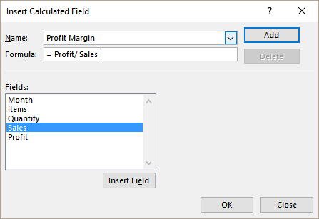
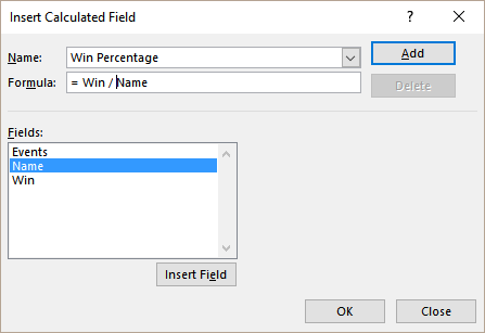
3. In the Insert Calculated Field dialog box,
   • Assign a name in the Name field.
   • In the Formula field, insert the formula =Profit/Sales by clicking on the Insert Field button from the Fields box.

4. Click ADD and then OK.

Limitation of the calculated fields in the pivot table when calculating a percentage

Calculated fields in pivot table have some limitations. A calculated field is always performed against the SUM of the data. This limits you from using a lot of functions. Furthermore, you cannot use any functions that require cell references or defined names as an argument. This rules out functions like COUNT, AVERAGE, IF, AND, NOT, and OR.

In the following example, you will use the Clayton High School Track and Field club’s event record for the past six months. It includes the Event, Names and Win records. You will calculate the count of wins as a percentage for the count of athletes based on the events.

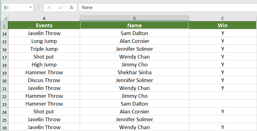
From this, we have the pivot table Count of Name and Count of Win.

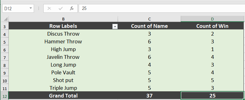
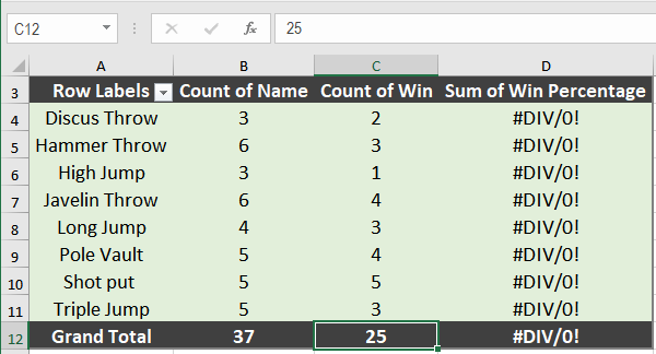
To find the count of wins as a percentage for the count of athletes based on events at first, you will try with a calculated field. Add a calculated field like the previous section named Win Percentage and having the formula =Win / Name.

As calculated field only performs calculations against the SUM of data, we get a #DIV/0 error.

To overcome this issue, you need to follow the next steps:

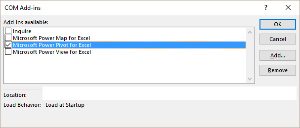
1. Make sure you have Power Pivot enabled in File > Options > Add-Ins.
2. Click COM Add-ins in the Manage box > Click Go.
3. Check the box for Microsoft Office Power Pivot > click OK. Select the Power Pivot add-in for Excel if you have other versions of power pivot installed.

From the Events_Record worksheet, go to Power Pivot > Manage.

You will use Data analysis expression (DAX) to create calculated fields in Power Pivot. DAX is used to add calculations. A measure is a formula that is created specifically for use in a pivot table that uses data in the Power Pivot. You will use the measure in the Values area of the pivot table.

1. In the Power Pivot window, Click Home> View> Calculation Area.

2. Click on an empty cell in the Calculation Area.
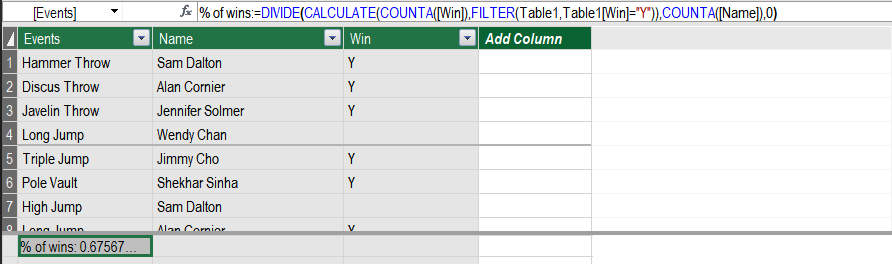
3. In the formula bar, at the top of the table, enter the formula,% of wins := DIVIDE(CALCULATE(COUNTA([Win]),FILTER(Table1,Table1[Win]="Y")),COUNTA([Name]),0)

4. Press Enter to accept the formula.

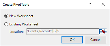
5. Click anywhere in the Power Pivot data. Go to Home > PivotTable.
6. In the Create PivotTable dialogue box, check New Worksheet.
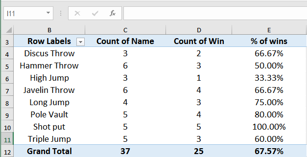
7. In the resulting pivot table worksheet, expand Table1 in the PivotTable Fields Menu on the right. Drag Events to the Row field. Name, Winand fx % of wins to the Values field.

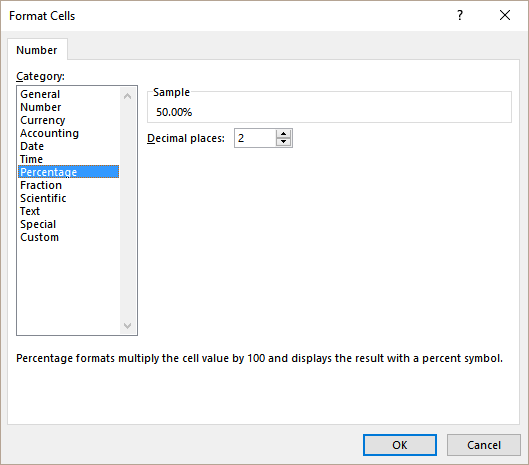
8. Right-click anywhere in the % of wins column in the pivot table. Select Value Field Settings > Show Values As > Number Format > Percentage. Click OK twice.

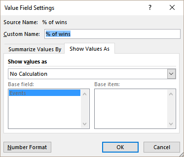
This will show the count of wins as a percentage for the count of athletes based on the events.

Pivot tables are a great way to summarize and aggregate data to model and present it. You can now visualize and report data in the blink of an eye. Dashboards and other features have made gaining insights very simple using pivot tables. Calculated fields in the pivot table is a great way to create formulas to add a sum of columns.

There are many powerful features of Pivot Tables, Power Pivot, and Data analysis expression (DAX) that could help you gain insights into your data. If you want to save hours of researching and frustration and get to the solution quickly, try our Excel Live Chat service! Our Excel experts are available 24/7 to answer any Excel question you have on the spot. The first question is free.