

We can create advanced Excel pivot tables to correlate different variables within our raw data. Pivot tables provide an exciting and quick approach to clean and format our data efficiently. The steps below will walk through the process.
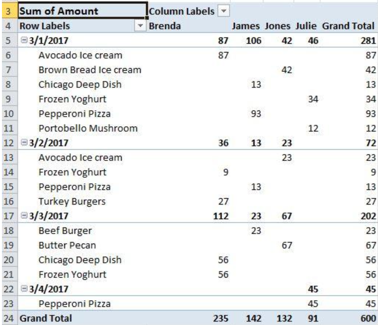 Figure 1- Example of An Advanced Pivot Table
How To Create an Advanced Excel Pivot Table
- We will create our data to show the sales made by a business in a particular period
- Our spreadsheet will contain the Sales Date, Category, Product, Quantity, Sales rep and amount in Columns A, B, C, D, E, and F respectively
 Figure 2 – Setting up the Data
- We will select any cell within our data
- In the Insert tab, we will click the Pivot table
- Within the Create Pivot table dialog, we will check that the data range is correct and click OK.
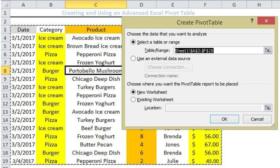 Figure 3 – Creating an Advanced Pivot Table
- We will now see an empty pivot table and to the right of the worksheet, a Pivot Table field list task pane. This is where we will assign our data fields.
![]() Figure 4 – An Empty Pivot Table Field List Task Pane
Figure 4 – An Empty Pivot Table Field List Task Pane
- We will drag the “Date” and “Product” field into the ROWS label
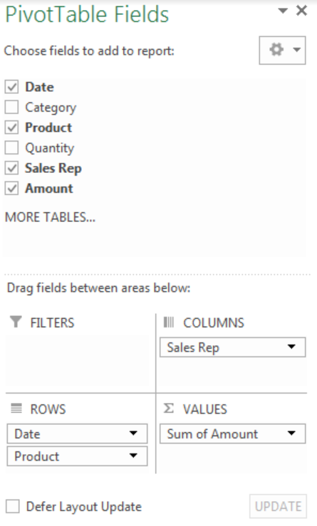 Figure 5.1- Pivot Table Fields
- Again, we will drag the “Amount” into the Values label
- Now, we will drag the Sales Rep into the Columns label
 Figure 5.2 – A Typical Advanced Excel Pivot Table
Quick Tips to Use Advanced Pivot Table Techniques in Excel
Slicers
We use slicers to refine the data in our Excel Pivot table so that we or other users can customize the pivot tables without difficulty and fast.
- To add a slicer, we will click within the Pivot table and check for the Analyze tab on the ribbon above our sheet.
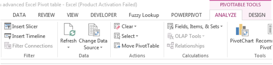 Figure 6.1 – Pivot Table tools to insert slicer
- We will click on Insert Slicer, select the slicers we want and click OK
 Figure 6.2 – Making a choice of the slicer
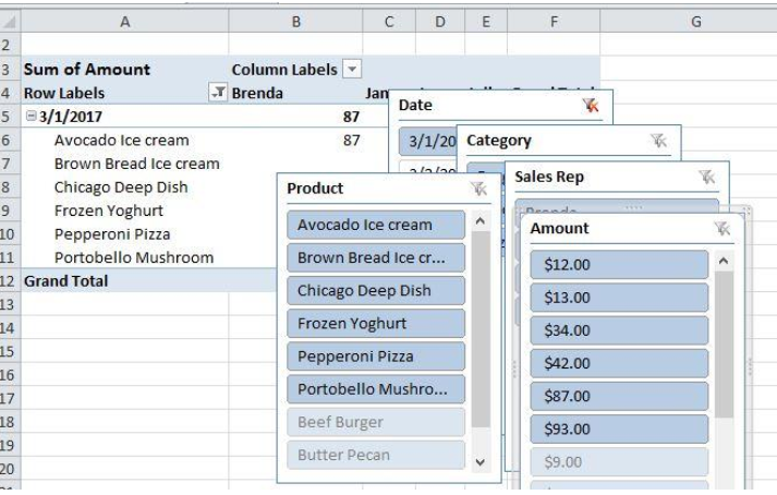 Figure 6.3 – Inserting Slicers
Timelines
When our data contains dates, we can use Timelines to select data from a specific period. We must ensure that our dates are formatted as a date in the spreadsheet.
- To add a timeline, we will select our Pivot table, click on Pivot table tools, and then, timeline. A window will pop up. Here, we can select the specific timelines we want to see.
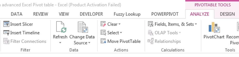 Figure 7.1 – Pivot Table tools to insert timeline
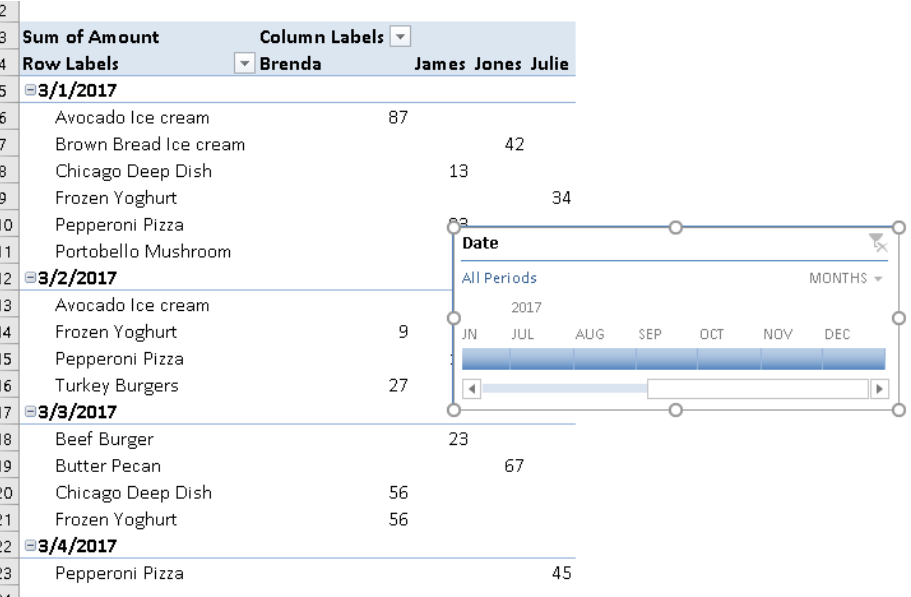 Figure 7.2 – Inserting Timelines
Tabular view
Sometimes, an excessive number of fields may cause issues with Excel when creating layers to write formulas on. We can view our pivot table in a tabular form rather than the default setting to allow us to write formulas on our data more efficiently.
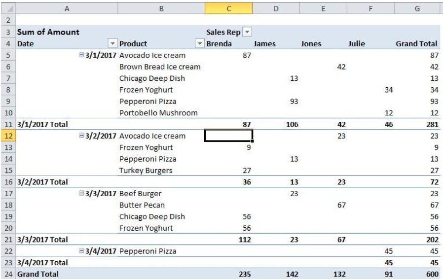 Figure 8 – Displaying Pivot Table in Tabular View
Calculated Fields
We can add a new column that wasn’t in our raw data into our pivot table with calculated fields.
- To get started with calculated fields, we will click on our Pivot table
- We will Click Analyze on the ribbon, then fields, Items & Sets and finally select calculated fields
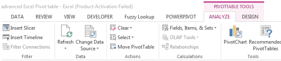 Figure 9.1- Clicking on Fields, Items & Sets
- In the pop-up window, we give our calculated field a name, such as Total Order Cost. We will enter the Total Order Cost formula given below into the allocated space, and click OK
=Amount*Quantity
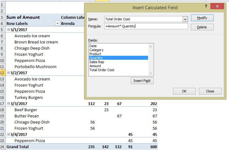 Figure 9.2 – Inserting Calculated fields
Recommended Pivot tables
We can use recommended pivot tables if we are confused about setting labels in our pivot table.
- We will highlight our data, go to the Insert tab and select Recommended Pivot Tables
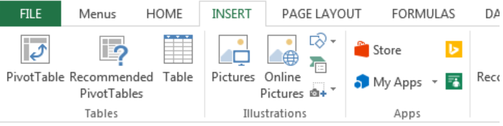 Figure 10.1 – Clicking on Recommended Pivot table
- In the popup window, we can click through the thumbnails on the left side to view the recommended Pivot table options
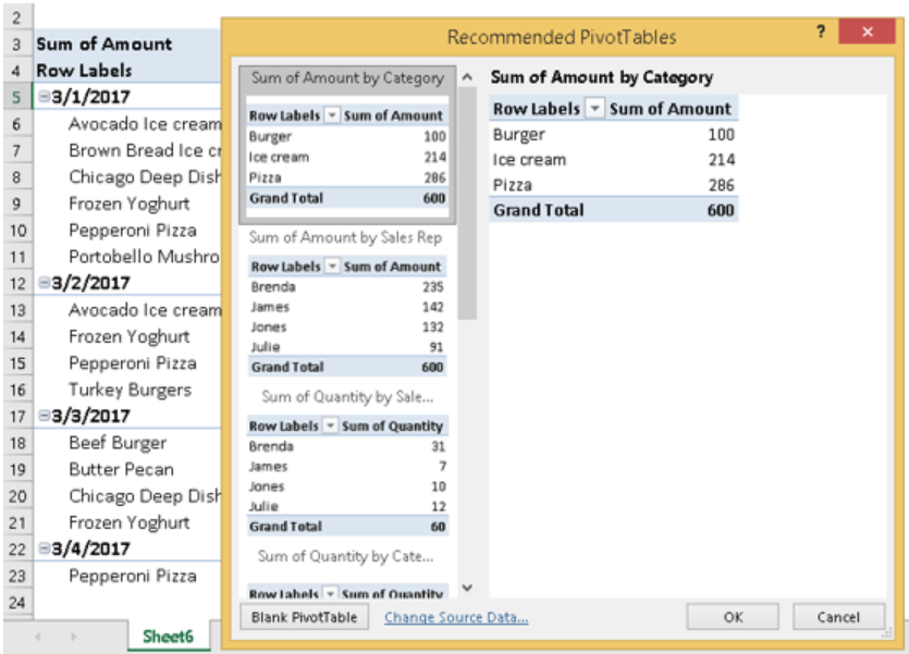 Figure 10.2 – Using Recommended Pivot tables
Most of the time, the problem you will need to solve will be more complex than a simple application of a formula or function. If you want to save hours of research and frustration, try our live Excelchat service! Our Excel Experts are available 24/7 to answer any Excel question you may have. We guarantee a connection within 30 seconds and a customized solution within 20 minutes.


Leave a Comment