

Have you ever found yourself in a situation where you have to choose an item from many alternatives? If yes, then you must know how tricky it is. In such a situation, you need to know how to do single factor ANOVA test popularly known as one way ANOVA test (Analysis of Variance).
One way ANOVA test is particularly important when we are faced with many things from which we want to select a single one. In this case, you have many options that are similar, and it is only way to know the best alternative is to run ANOVA.
Knowing how to perform ANOVA will help us make a confident and reliable decision. This is because one way ANOVA test presents us with the evidence to support the decisions we make. But how do we calculate ANOVA? This post will walk you through the steps necessary to do ANOVA.
Step-by-step guide on how to do ANOVA test
Step 1: Prepare the data for which you want to do analysis of variance
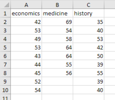 Figure 1: Data for ANOVA table
In figure 1 above, we have data pertaining to people’s salaries based on their degrees. The degrees are Economics, Medicine and History.
Step 2: Click Data Analysis
The next thing we need to do is head to the toolbar ribbon and click on the Data tab. We shall be presented with a window. In that window click Data Analysis.
 Figure 2: Click Data Analysis
But we need to be aware that not all MS Excel have the Data analysis button. If yours does not have this, then it will be quite hard to test ANOVA using Excel without loading it first. You need to load the Analysis ToolPak add-in before you proceed from this step.
Step 3: Select ANOVA
After loading the Data analysis tool, you will have the Data analysis button. Click on the button. This will present you with a popup window. In the window, select ANOVA: Single Factor. Then click OK.
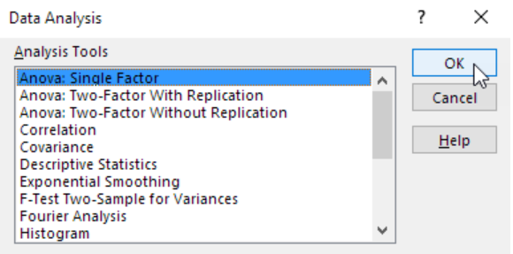 Figure 3: Select ANOVA single factor
Step 4: Input the range
We now have to input the range of values for which we want to do the one way ANOVA test. For our example, we shall have the range from A2:C10. We then click OK after putting in the range of values to calculate the single factor ANOVA.
Step 5: Output range
We need to select a cell as an output range. We have cell E1 for this purpose.
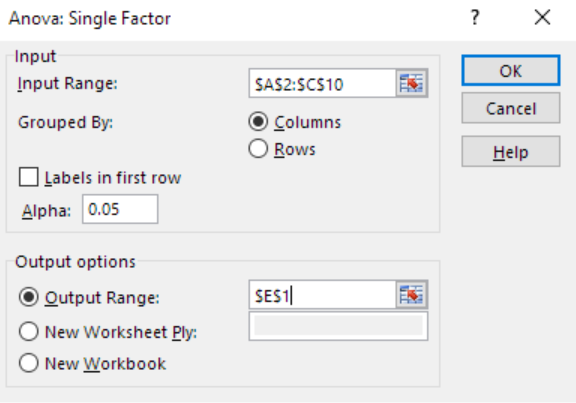 Figure 4: Choose output range
The click ok.
Check the result in an ANOVA table
You actually don’t have to know how to run ANOVA table. With all the above procedures having been followed, and you click OK, you will get an ANOVA table that contains the results. The software shall create the ANOVA table for us. For our example, we have the ANOVA table below with the results;
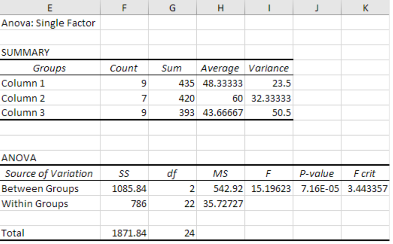 Figure 5: ANOVA table
ANOVA testing is as easy as that, but then we also have to know how to interpret the answer we get after carrying out ANOVA test in Microsoft Excel.
Interpretation of the results of ANOVA table
In the event that we get F > F critical, then we shall have to reject the null hypothesis. In our case, we have our F as 15.19623 while F critical is 3.443357. And given that 15.19623>3.443357, we have to reject the null hypothesis.
Rejection of the null hypothesis shall mean that the means of the three salaries are not equal. But one way ANOVA calculator does not tell us where this different lies. For this reason, we also have to know how to use the T-test.
Instant Connection to an Excel Expert
Most of the time, the problem you will need to solve will be more complex than a simple application of a formula or function. If you want to save hours of research and frustration, try our live Excelchat service! Our Excel Experts are available 24/7 to answer any Excel question you may have. We guarantee a connection within 30 seconds and a customized solution within 20 minutes.


Leave a Comment