In excel, it is possible to list the most occurring numbers based on four Excel functions that include the IF, MODE, MATCH and ISNUMBER functions. This article provides a guide on how we can use these functions to list the most frequently occurring numbers in excel.
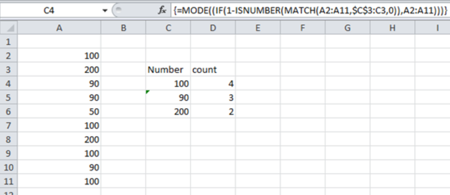
 Figure 1: How to get a list of most occurring numbers in Excel
General syntax of the formula
{=MODE(IF(1 – ISNUMBER(MATCH(data, exp_rng, 0)), data))}
Where;
Data- refers to the range where the numbers from which you want to find the most frequently occurring are located.
Understanding the formula
The formula above is critical when we want to get a list of most frequently occurring numbers in a given column. Note that this is an array formula, and thus if you want to get the correct result, you need to enter it using the array format, i.e. Control + Shift + Enter.
How the formula works
- This formula has four functions, the IF, MODE, MATCH and ISNUMBER functions
- Among these functions, the MODE function plays the most critical role of returning those numbers that have appeared the most number of times.
- The other functions are also vital, though not as much as the MODE function.
- They only help to create a filtered array for MODE to use for each of the rows.
- In our example above, you should have noticed $C$3:C3, which is referred to as the expanding range. This is used to exclude those numbers that already have their results in $C$3:C3.
Understanding the functions
In the formula, we have the following functions and the purpose they serve;
- MATCH function- the purpose of this function is to check all the numbers in the range, “data” against the existing numbers in the expanding range $C$3:C3
- ISNUMBER- this function is used to convert matched values to TRUE and those that do not match to FALSE
- 1- NUMBER- this one is used to reverse the array. Also, the math outputs ones and zeros
- IF– this uses the array output of result of 1-NUMBER to filter values in the original list. It excludes the $C$3:C3
- MODE- this functions then returns the most frequent number in the specified array.
Handling errors
In the event that in the array supplied there non-recurring numbers, the MODE function will return a #N/A error. We can use the IFERROR function to remove this error and replace it with empty strings. The formula will thus look like the one below;
=IFERROR(MODE(IF(1-ISNUMBER(MATCH(data, $C$3:C3,0)),data)), “ ”)
Example
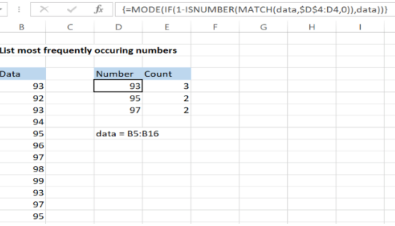
 Figure 2: Example of a list of most frequently occurring numbers
In this example, we want to list the most occurring numbers. To do this, proceed as follows;
Step 1: Prepare the list as shown in column B.
Step 2: Indicate where you want to get the results, as shown in column D and E
Step 3: Select the cells where you want the results to appear.
Step 4: Enter the formula relative to the active cell
Step 5: Press Control + Shift + Enter to enter the formula in an array form.
Instant Connection to an Expert through our Excelchat Service
Most of the time, the problem you will need to solve will be more complex than a simple application of a formula or function. If you want to save hours of research and frustration, try our live Excelchat service! Our Excel Experts are available 24/7 to answer any Excel question you may have. We guarantee a connection within 30 seconds and a customized solution within 20 minutes.


Leave a Comment