

Excel helps its users offering some great solutions for arithmetic operations. SUMPRODUCT is one such function. It multiplies ranges or arrays and returns the product sums.We can nest other functions inside the SUMPRODUCT function to enhance its ability. In this tutorial, we will learn how to use the SUMPRODUCT function in Excel.
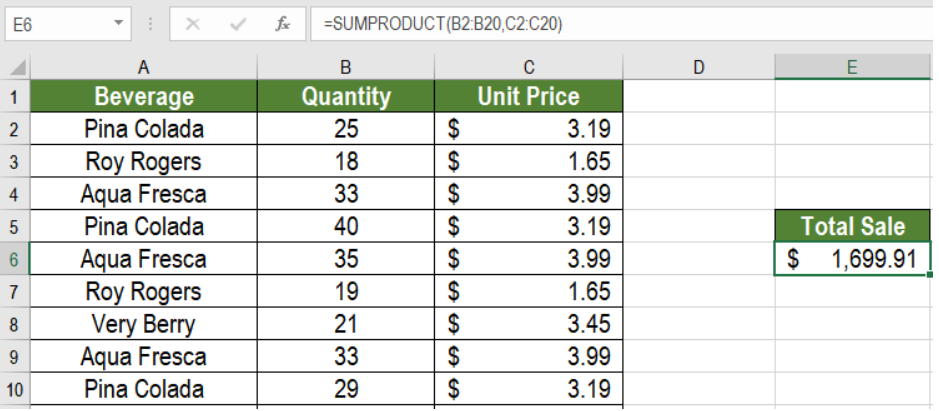 Figure 1. Example of the SUMPRODUCT Function in Excel
Syntax
=SUMPRODUCT (array1, [array2], ...)
- array1: This value is required. The first array to multiply, then sum.
- array2: This value is optional. The next array to multiply and add. SUMPRODUCT can take up to 30 arrays.
The SUMPRODUCT function multiplies and then sums the array values. Though it deals with arrays, it does not require Ctrl + Shift + Enter. SUMPRODUCT sums the array items if only one array is provided as the argument.
In the next part of this tutorial, we will see some uses of the SUMPRODUCT function.
Excel SUMPRODUCT Function to Multiply and Sum Arrays
The main use of the SUMPRODUCT function is to multiply and sum array entries. The following example contains a beverage sale data set. Column A, B and C has the names, quantity and unit price.
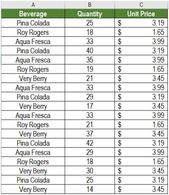 Figure 2. The Sample Data Set
To find out the total revenue in cell E6:
- We need to click cell E6.
- Assign the formula
=SUMPRODUCT(B2:B20,C2:C20)to E6. - Press Enter.
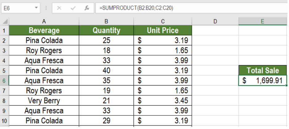 Figure 3. Applying the Formula to the Data
This will show the total revenue from the beverage sales in E6. Here, B2:B20 represents array1 and C2:C20 represents array2. SUMPRODUCT multiplies them and adds the result to find the sum.
Notes
- Excel returns #VALUE error if the arrays are not same in length.
- Non numeric values will be counted as zero (0).
- Booleans values will be converted into ones (1) and zeroes (0) using double negation.
Count Cells with Condition using the SUMPRODUCT Function
The SUMPRODUCT function in Excel can count cells based on conditions. It performs the same operations like the COUNTIF function but in a simpler way.
Syntax
=SUMPRODUCT(--(array=condition))
Here, SUMPRODUCT checks the array for every instance where the condition is met. It returns the boolean value TRUE if it is a match, else it returns FALSE. The double negation (–) translates the boolean values to ones (1) and zeroes (0). SUMPRODUCT only counts the ones. Thus, it returns the count where the condition is met.
To count the instances of the beverage Aqua Fresca from the last example:
- We need to go to cell F6.
- Assign the formula
=SUMPRODUCT(--(A2:A20=F5))to the formula bar or F6. - Press Enter.
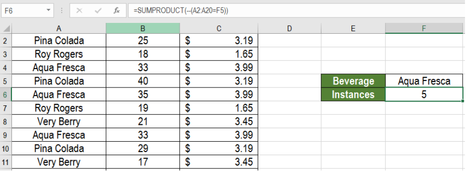 Figure 4. Applying the Formula to the Data
This will show the count of the Aqua Fresca instances from the data.
Sum Cells with Condition using the SUMPRODUCT Function
Sumproduct can also sum cells within an array based on a condition. It works the same way as the SUMIF function.
Syntax
=SUMPRODUCT(sum_range,--(criteria_range=criteria))
Here, SUMPRODUCT checks the array for every instance where the condition is met. Like the previous example, SUMPRODUCT returns TRUE and FALSE values depending on a match. We transform these values to ones (1) and zeroes (0) using the double negation operator (–). This array is then multiplied with the criteria_array. Now, only the ones with the match remains in the criteria_array.
Next, SUMPRODUCT multiplies the values in the criteria_array with the corresponding values from the sum_array and returns the result.
To find the total sales of the beverage Verry Berry from the last example:
- We need to go to cell F6.
- Assign the formula
=SUMPRODUCT(C2:C20*B2,--(A2:A20=F5))to the formula bar or F6. - Press Enter.
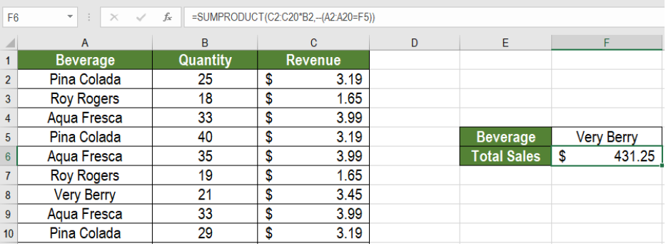 Figure 5. Applying the Formula to the Data
This will show the total sales of Very Berry in cell F6.
Most of the time, the problem you will need to solve will be more complex than a simple application of a formula or function. If you want to save hours of research and frustration, try our live Excelchat service! Our Excel Experts are available 24/7 to answer any Excel question you may have. We guarantee a connection within 30 seconds and a customized solution within 20 minutes.


Leave a Comment