

We can use the excel RANDBETWEEN function to generate random numbers in excel. The steps below will walk through the process.
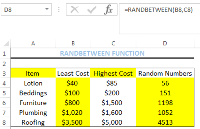 Figure 1: Result of RANDBETWEEN function for Cells of Column D
General Formula
=RANDBETWEEN(bottom,top)
- Bottom – This is the smallest random integer that will be returned by the RANDBETWEEN function. It is the lowest value in the range.
- Top – This is the largest random integer that will be returned by the RANDBETWEEN function. It is the highest value in the range.
Formula
=RANDBETWEEN(B4,C4)
Setting up the Data
- We will set up the data by inputting the LEAST COST and HIGHEST COST into Column B and Column C respectively
- Column D is where we want the formula to return the result for the random numbers
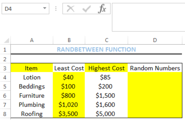 Figure 2: Setting up the Data
Getting the Random Numbers
- We will click on Cell D4
- We will insert the formula below into the cell
=RANDBETWEEN(B4,C4)
- We will press the enter key
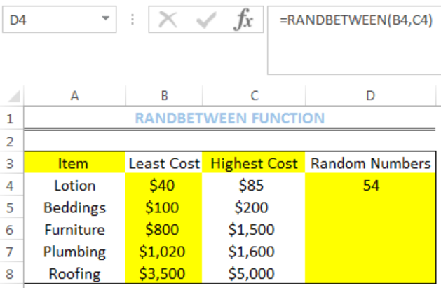 Figure 3: Result of RANDBETWEEN function for Cell D4
- We will click on Cell D4 again
- We will double-click on the fill handle (the small plus sign at the bottom right of Cell D4) and drag down to copy the formula into the other cells
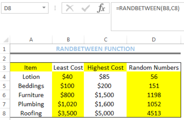 Figure 4: Result of RANDBETWEEN function for Cells of Column D
Notes
- RANDBETWEEN function generates a new random number if you click on an existing cell with the formula
- RANDBETWEEN function generates a new random number after every recalculation
- To retain random numbers, press the F9 button after using the RANDBETWEEN function in the cell.
Instant Connection to an Expert through our Excelchat Service
Most of the time, the problem you will need to solve will be more complex than a simple application of a formula or function. If you want to save hours of research and frustration, try our live Excelchat service! Our Excel Experts are available 24/7 to answer any Excel question you may have. We guarantee a connection within 30 seconds and a customized solution within 20 minutes.


Leave a Comment