How to use the Excel MROUND function

Excel MROUND Function

We use the MROUND function to round off a given set of numbers either up or down to the nearest specified multiple. The steps below will walk through the process.

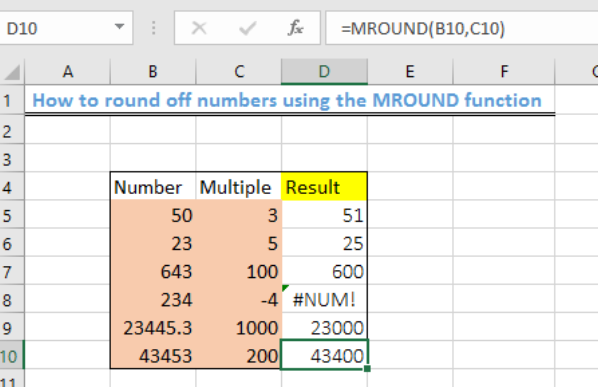Figure 1- Result of rounding off numbers using the MROUND function

General formula

=MROUND(num,multiple)

Formula

=MROUND (B5,C5)

Setting up the Data

The objective is to round off each number using the multiples as shown in figure 2

We will input the numbers in the range B5:B10 and titled them as “Number.”
We will put the multiples in C5:C10 and title them as “Multiple.”
Column D will contain the results after applying the MROUND function

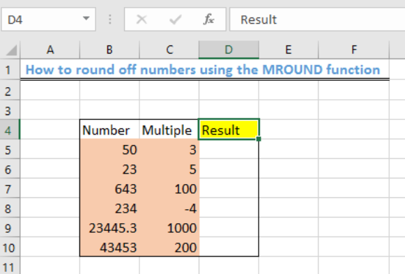Figure 2- Setting up the Data

Applying the MROUND function

We will click on Cell D5

We will insert the formula: =MROUND (B5,C5) into Cell D5

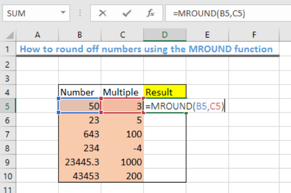Figure 3 – Applying the MROUND function

We will press the Enter key

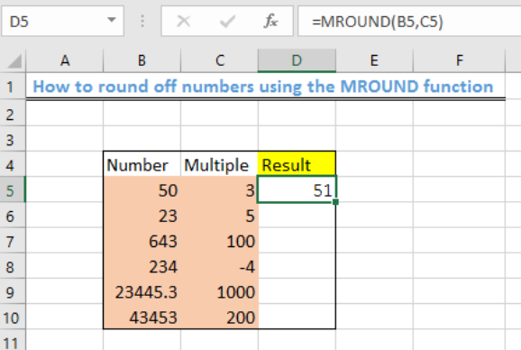Figure 4- How to round off numbers using MROUND function

Using the fill handle, we will copy the formula to the other cells of the Result column

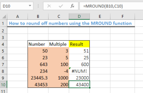Figure 5 – Result of rounding off numbers using the MROUND function

Explanation

=MROUND (num,multiple)

The MROUND function rounds off numbers (“num”) to the nearest multiple that is specified. The MROUND function always rounds away from zero and the rounding will occur if the remainder from the left when dividing the number by the multiple is greater than or equal to half of the multiple values. Multiple must also have the same sign as the number. If the numbers and multiples do not have the same sign, then the #NUM error will be displayed as shown in figure 4, Cell D8.

Instant Connection to an Expert through our Excelchat Service

Most of the time, the problem you will need to solve will be more complex than a simple application of a formula or function. If you want to save hours of research and frustration, try our live Excelchat service! Our Excel Experts are available 24/7 to answer any Excel question you may have. We guarantee a connection within 30 seconds and a customized solution within 20 minutes.

Did this post not answer your question? Get a solution from connecting with the expert.

Another blog reader asked this question today on Excelchat:

Hello, i am trying to create a formula to bundle posts into bundles of 25, and give a quantity of bundles, currently i have this =IF($G10,(MROUND(G10/25,1)),"1") G10 is number of tubes in a bundle. with the current function if the number of tubes is less than 13 the number of bundles is 0. when it needs to be if less than 25 = 1 any chance you can help?

An Excelchat Expert solved this problem in 26 mins!

1.Rename the template with your last name, delimited by a comma, a space and then your first name, e.g. Doe, Janenotice the capitalization.Note: changing the file extension from .xlsm to .xlsx or disabling the embedded macro or deleting its results will result in major point deductions! You need to start completely over from the original .xlsm file if you renamed it or if you get a Microsoft Visual Basic run-time error 9 (subscript out of range).2.Open the Excel workbook.3.If you see a Microsoft Excel Security Notice popup. If so, click the Enable Macrobutton and continue, i.e. you must enable macro when the template first open.4.If you see a yellow Security Warning banner underneath the Ribbon (row of tabs and buttons), click either the Enable Content button (or the Option...button and then select the radio for Enable this content follow by clicking the OK button).5.In case the Unit Forecast tab is not on top, click on the Unit Forecast tab on the bottom of the Excel window to put the focus on that worksheet.When you turn in your workbook, the Unit Forecast tab needs to be on top with the workbook opens.6.Personalize your workbook by entering your personal information in cells B1 throughB4, and then delete the text in B5 that does not pertain to your class section.Dont worry if Excel thinks that the content is a hyperlink and turn the font color to blue or something other than blank.Everything that you enter into B1 through B5 in the Unit Forecast worksheet will show up automatically in the corresponding cell in the Income Statement IS 312Project #1: ExcelDavid Liu, Ph.D.Page 2of 5This is an academic assignment: Report all unethical conduct to david.liu@csun.eduworksheet.IMPORTANT: SAVE your file at this point and DO NOT change the file type (e.g. by using the SAVE AS open instead of just SAVE). If you do (at any point of the project), start from the version before made this mistake. Otherwise, your project grade for the project could be greatly penalized.7.Find the cells for forecasting unit sales for the 3 products along 8 consecutive quarters.8.The 1st quarter unit sales of Product A Basic Edition is the basis for ALL other unit forecast.9.Quarter-over-quarter unit growth is expected to be 10% with the exceptions of the 4th quarter in each year. Generally, a 30% spike is expected in the 4th quarter instead of the normal10%quarter-over-quarter unit growth. For the 1st quarter of year 2, the growth rate goes back to10% and then spikes to 30%again on the 4th quarter of the 2nd year.10.If your method of calculation for quarter-over-quarter unit growth can be done with a single formula over the entire 8 quarters, you will earn extra points. One way to do this is to use a combination of functions such as IF and LEFT. But dont concern yourself with this until you have complete all the requirements, then come back to make an attempt at this. It is extra work for extra points.11.Apply horizontal references first before vertical references. In other words, work within each product category and not within a quarter across the three products.The open exception is the 1st quarter of the 1st year because there are no other options. 12.Product A Premium Edition unit sales is only 50% of that of the Basic Edition. However, the Premium Edition sells for 5 times the price of the Basic Edition. Reminder: price only comes into the calculations on the Income Statement worksheet.13.Product B unit sales is the same as Product A Basic Edition, but sells for twice the price of Product A Basic Edition.14.The 1st quarter staff head count is the basis for all other quarters staffing forecast.Note that this does not apply to the executive head counts because those numbers are already given on the template.15.Starting at the 2nd quarter of the 1st year, a steady 5% staffing expansion is expected each quarter over the two-year period. MROUND all the cells(including the very 1st quarter)that contain staffing head counts to a quarter of a person (.00, .25, .50 or .75).16.Commission is 20% of sales revenue.17.COGS is 40% of sales revenue. 18. The five yellow highlighted cells in the template drive the calculation of the entire workbook. To set up the automatic calculations on the gray color cells, your formulas are to reference these five yellow highlighted cells or their derivatives.Do NOT remove the yellow highlight formatting from these five cells.19.The numbers for the Income Statement (i.e. the second worksheet) are derived from numbers in theUnit Forecast (i.e. the first worksheet). It is important for you to use referenced values rather than manually entering numbers into each cell. By using referenced value, changes will automatically propagate as appropriate.20.Once you have inputted all your formulas, you are to pick random numbers of your own choosing and enter them into those five yellow highlighted cells to validate your calculations.Note: you can also check with your neighbor to see if your formulas generate the same results. If you the results are the same, then either you are both right or you are both made the same mistakes.If they are different, then you and your neighbor had different formulas.

An Excelchat Expert solved this problem in 21 mins!

Post your problem and you'll get expert help in seconds