How to Use VLOOKUP with Numbers and Text

If we want to use the VLOOKUP function with both numbers and text, there usually is a mismatch between numbers and text. This article will step through the process of successfully using the VLOOKUP function with number and text.

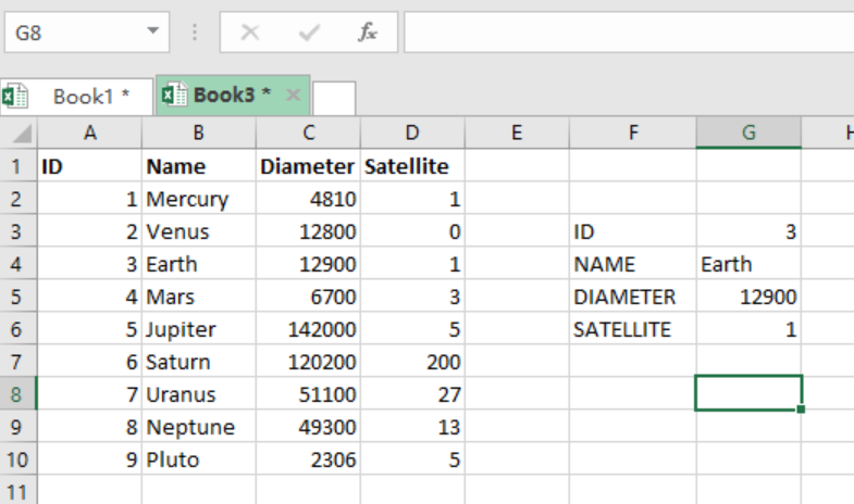
Figure 1. Final result

Formula

Below are the original and revised forms of the formula.

=VLOOKUP(id, planets, 2, 0) // Original

=VLOOKUP(id &””, planets, 2, 0) // Revised

How the function works

Concatenating an empty string to a number converts it to text. This can also be done with a longer formula which utilizes the TEXT function to convert to text.

=VLOOKUP(TEXT(id, “@”), planets, 2, 0)

Even with these formulas, we might still be unsure whether we are dealing with numbers or text. In such an instance, we need to wrap the VLOOKUP formula inside IFERROR. This will yield the formula below:

=IFERROR(VLOOKUP(id, planets, 3, 0), VLOOKUP(id&””, planets, 3, 0))

Example 1: VLOOKUP with numbers and text

Step 1: Prepare the data

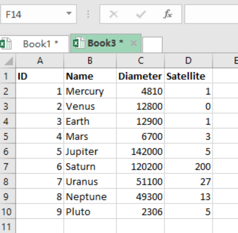
Figure 2. Example on how to use VLOOKUP with Numbers and Text

Step 2: Specify where to put the formula then Press Enter.

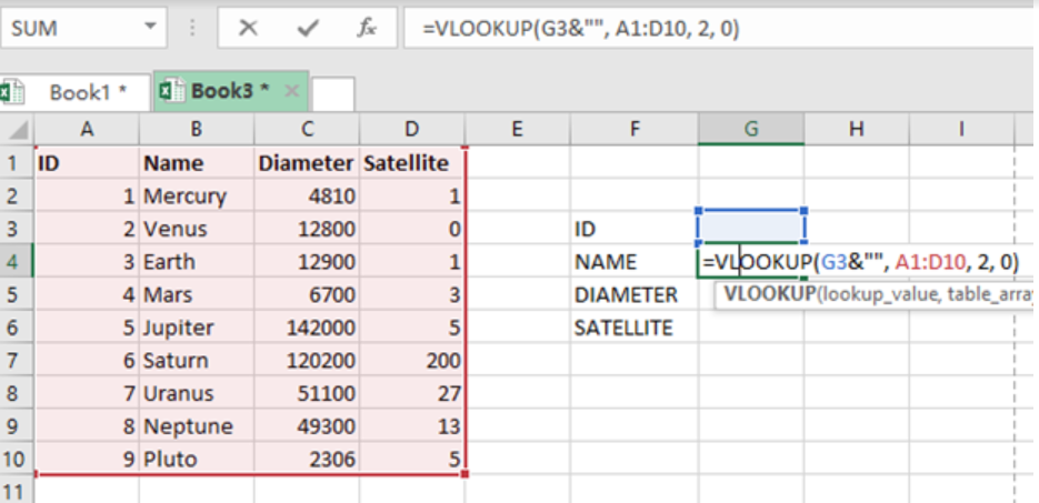
Figure 3. Example on how to use VLOOKUP with Numbers and Text

Your final result should be as below:

Figure 4. Example on how to use VLOOKUP with Numbers and Text

Instant Connection to an Expert through our Excelchat Service

Most of the time, the problem you will need to solve will be more complex than a simple application of a formula or function. If you want to save hours of research and frustration, try our live Excelchat service! Our Excel Experts are available 24/7 to answer any Excel question you may have. We guarantee a connection within 30 seconds and a customized solution within 20 minutes.

Are you still looking for help with the VLOOKUP function? View our comprehensive round-up of VLOOKUP function tutorials here.