

We can use a nested formula that combines the VLOOKUP and HLOOKUP Functions in excel to retrieve values from a table. Approximate and exact matching is supported by this combined formula and wildcards (* ?) are for finding partial matches. The steps below will walk through the process.
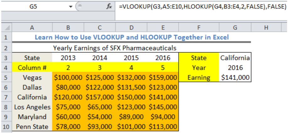 Figure 1- How to Use VLOOKUP and HLOOKUP Together in Excel
Syntax
=VLOOKUP(lookup_value,lookup_array,HLOOKUP(lookup_value ,lookup_array,2,range_lookup),range_lookup)
- Lookup_Value: This is the value to search for
- Lookup_array: This is the range to search for the lookup value
- HLOOKUP: This serves as the COLUMN NUMBER in the VLOOKUP formula. It specifies the COLUMN where we retrieve the data
- Range_lookup: This is used to specify if we want an approximate or exact match. If omitted, an approximate match is used
Formula
=VLOOKUP(G3,A5:E10,HLOOKUP(G4,B3:E4,2,FALSE),FALSE)
Setting up the Data
- We will use the combined formula to find the earning of California in 2016.
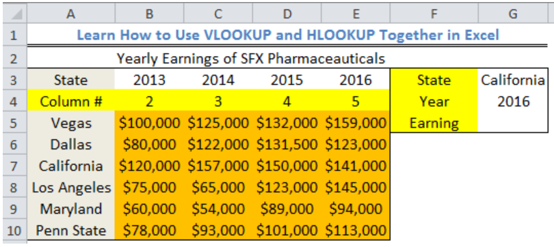 Figure 2 – Setting up the Data
Using the VLOOKUP and HLOOKUP Functions
- We will click on Cell G5
- We will insert the formula below into Cell G5
=VLOOKUP(G3,A5:E10,HLOOKUP(G4,B3:E4,2,FALSE),FALSE) - We will press the enter key
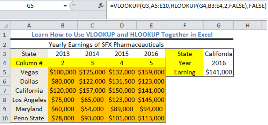 Figure 3- Result of the VLOOKUP and HLOOKUP Functions
Explanation
In this formula, the horizontal value (2016) is looked up with the HLOOKUP section of the formula. The returned value by HLOOKUP is 5 because HLOOKUP searches for 2016 in the range B3:E4 in ROW 2.
The vertical lookup value (California) is searched for by VLOOKUP. VLOOKUP searches the range A5:E10 for what is contained in Cell G3. After identifying California in the range, it then matches California with the returned column value (5) by HLOOKUP and returns $141,000.
Note
- If the lookup_value is greater than every value in the lookup table, the formula returns with the last value provided it has been set to approximate match
- If the lookup_value is less than all values in the lookup table, the function returns the #N/A error
- If we omit range_lookup, both functions will allow a non-exact or approximate match, but it will use an exact match if one exists. The approximate match is set as 1 and exact match is set as 2.
- If we set the range_lookup to approximate match, then the lookup values in the first row of the table must be sorted in ascending order. Otherwise, HLOOKUP may return an incorrect or unexpected value.
- If range_lookup is FALSE (exact match), values in the first row of the table do not need to be sorted.
This formula can only be used when the data is in a matrix form.
Instant Connection to an Expert through our Excelchat Service
Most of the time, the problem you will need to solve will be more complex than a simple application of a formula or function. If you want to save hours of research and frustration, try our live Excelchat service! Our Excel Experts are available 24/7 to answer any Excel question you may have. We guarantee a connection within 30 seconds and a customized solution within 20 minutes.


Leave a Comment