

There are times when we want to lookup a value in an excel table using both the rows and columns. To do this, we need to build a formula that is based on a two-way lookup with INDEX and MATCH as explained in this article.
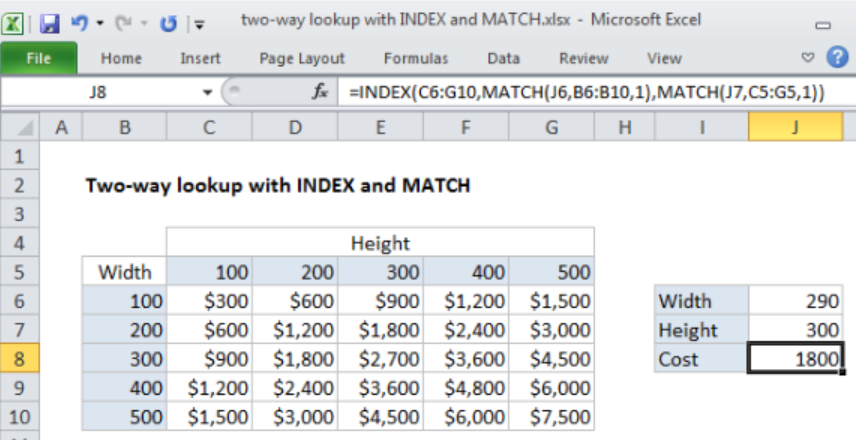 Figure 1: How to do two-way lookup with INDEX and MATCH
General syntax of the formula
=INDEX(data, MATCH(val,rows,1),MATCH(val,columns,1))
How the formula works
- This formula carries out approximate match. This means that you need to first sort the data before you apply it.
- The INDEX function forms the backbone of the formula. This function retrieves the value from the data as supplied in range C6:G10. This is based on a row number as well as column number.
- This is in the following form; =INDEX(C6:G10, row, column)
- The MATCH function then comes in to help get the row and column number. This function is also configured to approximate match by setting the third argument to 1, implying TRUE.
Example
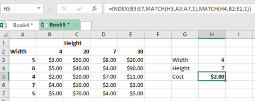 Figure 2: Example of how to do two-way lookup with INDEX and MATCH
In the above example, we want to find the cost of at the point where the height 7 and width 4 meet. To do this, we proceed as follows;
Step 1: Tabulate the excel table with data
Step 2: Indicate where you want the data to be located, i.e. in column H.
Step 3: Indicate the parameters, i.e. the width (4) and the height (7).
Step 4: Then in the cell where we want to have the cost, we put the formula =INDEX(B3:E7,MATCH(H3,A3:A7,1),MATCH(H4,B2:E2,1))
Step 5: We press Enter to get the cost as $2.00
Instant Connection to an Expert through our Excelchat Service
Most of the time, the problem you will need to solve will be more complex than a simple application of a formula or function. If you want to save hours of research and frustration, try our live Excelchat service! Our Excel Experts are available 24/7 to answer any Excel question you may have. We guarantee a connection within 30 seconds and a customized solution within 20 minutes.


Leave a Comment