How to Find a Partial Match Against Numbers with a Wildcard in Excel

The Wildcard character is used to signify a dummy character to substitute the actual character in the text. So, ultimately you won’t need to search the actual text but can look up the partial text.

What is a Partial match against numbers with a wildcard in Excel?

The Partial Match against numbers with the wildcard is done to employ criteria of searching the partial match of the text.

How the Partial match against numbers with the wildcard is used in Excel

The use of the Partial match against numbers with the wildcard is used to perform the partial match against numbers. Hence, you must use the MATCH and TEXT functions for the lookup. The working of the function is explained in the Example.

Formula or Syntax using MATCH

The formula that must be used is

{=MATCH(“*”&number&”*”,TEXT(range,“0”),0)}

Parameters or Arguments of a Partial match against numbers with wildcard

The arguments that must be passed in the function are:

•         Lookup_value: Required. This is the value to be matched in the array.
•         Lookup_array: Required. It is the range of cells or array reference.
•         Match_type: Optional. It is the criterion which is used for the match, specified as -1, 0, or 1.
•         Format_text: Required. It defines the number format that must be used in the lookup.

Example:

We will consider a direct example to perform a partial match against numbers with a wildcard:

1. Construct a table of several numbers and use the array formula based on the MATCH and TEXT functions.

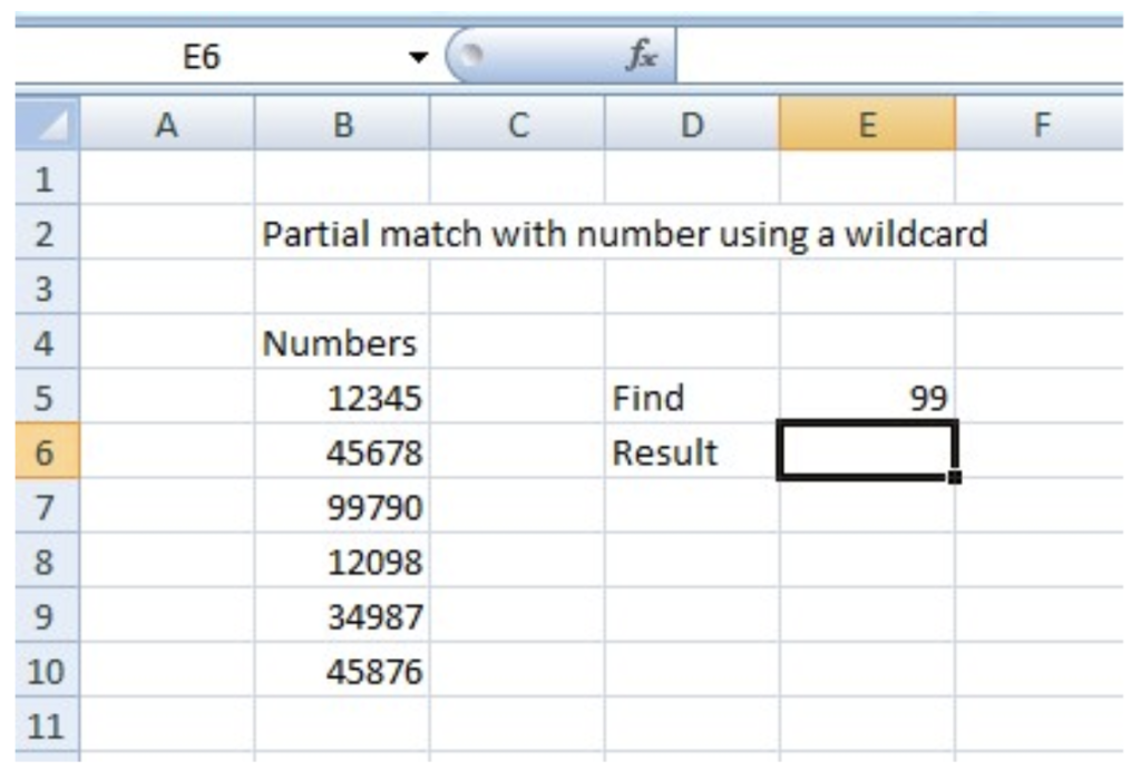Figure 1. Construct a table with several numbers

2. You have an option to convert the lookup range to text values if you want to perform a normal lookup with the MATCH and VLOOKUP functions. But, there is another option to use the TEXT function to convert the values within the formula.

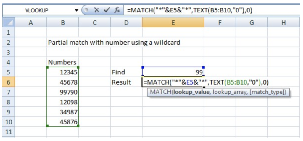Figure 2. Insert the MATCH and TEXT function

3. Now, use the formula as =MATCH (“*”&E5”*”, TEXT (B5: B10, ”0”), 0) and press Control+ Shift+ Enter to apply the array formula. The TEXT function will transform the numbers into text, and the MATCH function will find the partial match. The Return will be given in the respective field as shown in the figure.

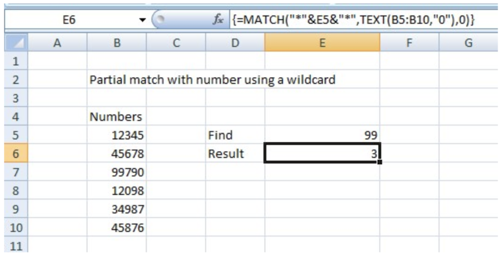Figure 3. The Return value will be given in Result Cell

Notes on Usage of the Partial match against numbers with wildcard

The note on usage is given below:

•         The default value of the Match type is 1.
•         The match function gives the relative position of the item we are trying to find in the array.
•         The TEXT function is useful when you want to embed the numeric output of a formula and represent it in some other format inside a text.
•         The Format_text must appear in the quotation marks.

Still need some help with Excel formatting or have other questions about Excel? Connect with a live Excel expert here for some 1 on 1 help. Your first session is always free.