

We can use the MATCH function to lookup the next largest match in a given set of values. This function is used in an approximate match mode, with -1 being for the match type. This post provides a clear guide on how to use the MATCH function to lookup the next largest match in a set of values.
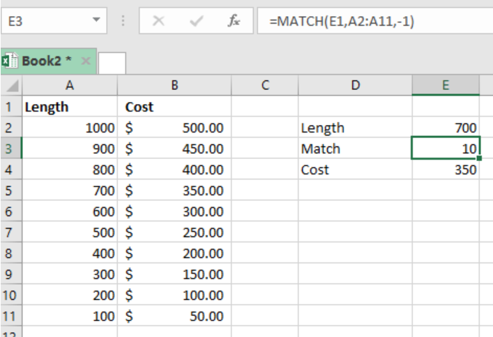 Figure 1. Final result
Syntax of the formula
=MATCH (value, array, -1)
Explanation
Normally, the MATCH function matches the next smallest value in a given list which has been arranged in an ascending order. It will then move to the next larger value than the lookup value, and then drop back to the previous value. When values have been sorted in an ascending order, the formulas below will return “next smallest”:
=MATCH (value, array) // default
=MATCH (value, array, 1) // explicit
The MATCH function will return the next largest match if the match type is set to -1, and the values arranged in a descending order.
In our example above, we have the formula in cell E3 as;
=MATCH(E1,A2:A11,-1)
Note that length is A2:A11, while cost is B2:B11.
Things to remember
While utilizing the match function, the following things are necessary to remember;
When the value set has been sorted in an ascending order, we shall need a match_type 1 at the end.
If the value set does not need any sorting, then you need a match_type 0.
We use a match_type -1 when the value set we are dealing with has been sorted in a descending order.
Instant Connection to an Expert through our Excelchat Service
Most of the time, the problem you will need to solve will be more complex than a simple application of a formula or function. If you want to save hours of research and frustration, try our live Excelchat service! Our Excel Experts are available 24/7 to answer any Excel question you may have. We guarantee a connection within 30 seconds and a customized solution within 20 minutes.


Leave a Comment