

We can now match the next highest value in a lookup table using a formula that is based on INDEX and MATCH functions. To learn how this is done, read this post to the end.
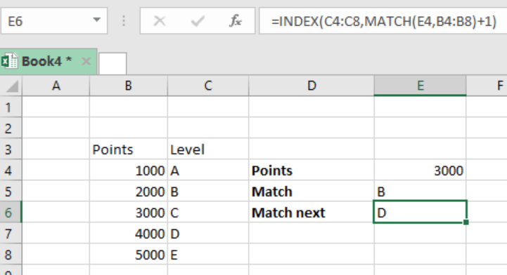 Figure 1: How to match next highest value with MATCH and INDEX
General syntax of the formula
=INDEX(data, MATCH(lookup, values)+1)
Where;
- Level- is the named range, A4:A8
- Data- is the named range B4:B8
How the formula works
- The formula has all the features of INDEX + MATCH.
- Here, the MATCH is utilized to find the correct row number for the value specified, which in our case is value in cell E4. In the absence of the third argument, match_type, the MATCH function will approximate match based on its default settings and will return 2.
- Note also that the level range is supplied in an array format. With 3 as the row number, the INDEX function will return “D” as the next highest value.
Instant Connection to an Expert through our Excelchat Service
Most of the time, the problem you will need to solve will be more complex than a simple application of a formula or function. If you want to save hours of research and frustration, try our live Excelchat service! Our Excel Experts are available 24/7 to answer any Excel question you may have. We guarantee a connection within 30 seconds and a customized solution within 20 minutes.


Leave a Comment