Lookup lowest value

While working with Excel, we are able to retrieve a value from a dataset through lookup based on a lowest value by using the INDEX, MATCH and MIN functions.  This step by step tutorial will assist all levels of Excel users to look up a value based on a lowest value in a data set.  

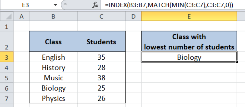Figure 1. Final result: Lookup lowest value

Final formula: =INDEX(B3:B7,MATCH(MIN(C3:C7),C3:C7,0))

Syntax of the INDEX function

The INDEX function returns a value as specified from within a range.

=INDEX(array, row_num, column_num)

The parameters are:

• array – a range of cells where we want to retrieve some data
• row_num – the row in the array from which we want to retrieve data
• column_num – the column in the array from which we want to retrieve data; if the array has only one column, column_num can be omitted

Syntax of the MATCH function

The MATCH function returns the position of a value in a range.

=MATCH(lookup_value, lookup_array, [match_type])

The parameters are:

• lookup_value – a value which we want to find in the lookup_array
• lookup_array – the range of cells containing the value we want to match
• [match_type] – optional; the type of match; if omitted, the default value is 1; We use 0 to find an exact match

Syntax of the MIN function

The MIN function returns the lowest value in a data set.  

=MIN(number1, [number2], ...)  

The parameters are:

• number1, number2, … – the numbers for which we want to find the lowest value; only number1 is required; succeeding numbers are optional
• The arguments could be numbers, array or reference to cells containing numbers

Setting up Our Data

Our table contains a list of Class (column B) and number of Students (column C). In cell E3, we we want to determine the class with the lowest number of students.  

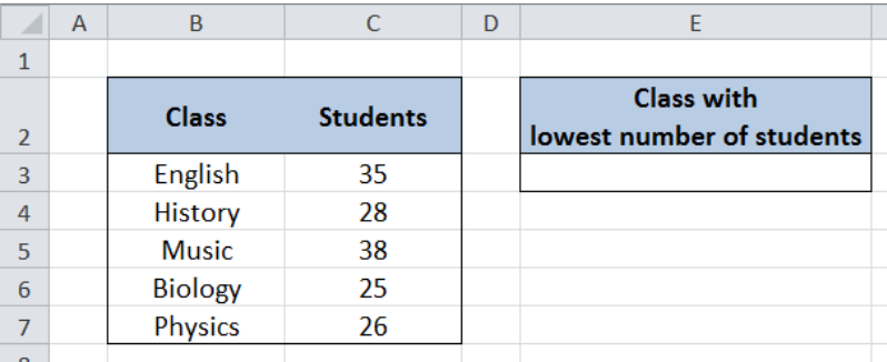Figure 2. Sample data to lookup lowest value

Lookup Lowest Value

In order to determine the specific class with the lowest number of students, we follow these steps:

Step 1.  Select cell E3

Step 2.  Enter the formula: =INDEX(B3:B7,MATCH(MIN(C3:C7),C3:C7,0))

Step 3: Press ENTER

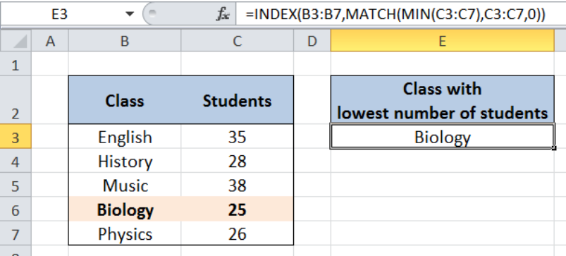Figure 3. Using INDEX, MATCH and MIN to lookup the class with lowest students

Our array for the INDEX function is the range B3:B7 which contains our data for “Class”.  The row number is determined through the MATCH and MIN functions.  

First, the MIN determines the lowest value for number of students, which is 25.  The MATCH function then returns the position of “25” in the range C3:C7, which is 4.  Hence, the row number is 4.  The column number is 0 since there is only one column in our array B3:B7.   

As a result, our formula returns “Biology” in cell E3, which is the class with the lowest number of students, and positioned in row 4 of the range B3:B7.  

Most of the time, the problem you will need to solve will be more complex than a simple application of a formula or function. If you want to save hours of research and frustration, try our live Excelchat service! Our Excel Experts are available 24/7 to answer any Excel question you may have. We guarantee a connection within 30 seconds and a customized solution within 20 minutes.