

Excel allows a user to do a two-dimensional lookup using the INDEX and MATCH functions. The MATCH function returns a row and a column for values in a table, while the INDEX returns a value for row and column. This step by step tutorial will assist all levels of Excel users to learn how to perform a two-dimensional lookup in Excel.
 Figure 1. The final result of the formula
Syntax of the INDEX formula
The generic formula for the INDEX function is:
=INDEX(array, row_num, column_num)
The parameters of the INDEX function are:
- array – a range of cells where we want to get a data
- row_num – a number of a row in the array for which we want to get a value
- column_num – a column in the array which returns a value.
Syntax of the MATCH formula
The generic formula for the MATCH function is:
=MATCH(lookup_value, lookup_array, [match_type])
The parameters of the MATCH function are:
- lookup_value – a value which we want to find in the lookup_array
- lookup_array – the array where we want to find a value
- [match_type] – a type of match. We put 0 as we want the exact match.
Setting up Our Data for the Formula
Our table is the matrix representing Sales per month and product. In column B, we have products and in the third row, we have months. In the range C4:G8, we have monthly sales per product. In the cells J2 and J3 we have the month and the product for which we want to get the Sales in J4.
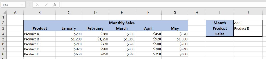 Figure 2. Data that we will use in the example
Performing a Two-Dimensional Lookup in Excel
We want to get the Sales for April (J2) and Product B (J3) in the cell J4. This data has to be looked up in the table C4:G8.
The formula looks like:
=INDEX(C4:G8, MATCH(J3, B4:B8, 0), MATCH(J2, C3:G3, 0))
The first MATCH function has lookup_value J3, lookup_array B4:B8 and match_type 0. The result of this function is the row_num parameter of the INDEX function. The second MATCH function has lookup_value J2, lookup_array C3:G38 and match_type 0. The result of this function is the column_num parameter of the INDEX function. The array parameter is the range C4:G8.
To apply the formula, we need to follow these steps:
- Select cell J4 and click on it
- Insert the formula:
=INDEX(C4:G8, MATCH(J3, B4:B8, 0), MATCH(J2, C3:G3, 0)) - Press enter.
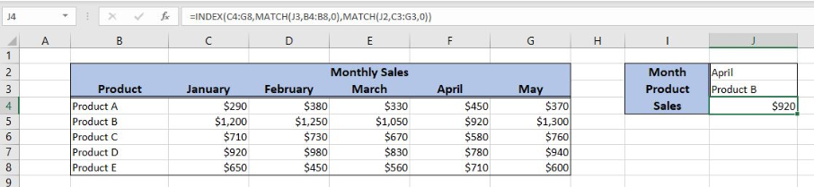 Figure 3. Using the formula to perform a two-dimensional lookup
The first MATCH function returns 2, as “Product B” is in the second place in array B4:B8. The second MATCH returns 4, as “April” is in the 4 places in array C3:G3. Therefore, the INDEX function returns the value in the second row and fourth column from the range C4:G8. The result in J3 is $920.
Most of the time, the problem you will need to solve will be more complex than a simple application of a formula or function. If you want to save hours of research and frustration, try our live Excelchat service! Our Excel Experts are available 24/7 to answer any Excel question you may have. We guarantee a connection within 30 seconds and a customized solution within 20 minutes.


Leave a Comment