

Excel allows a user to do a multi-column lookup using the INDEX and MATCH functions. The MATCH function returns a row for a value in a table, while the INDEX returns a value for that row. This step by step tutorial will assist all levels of Excel users in learning tips on performing a multi-column lookup.
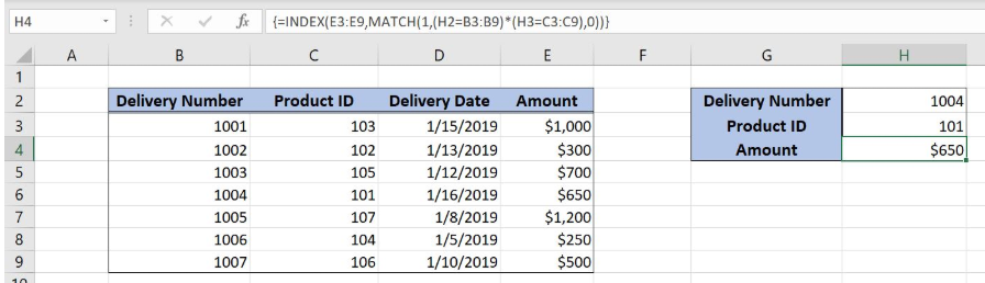 Figure 1. The final result of the formula
Syntax of the INDEX formula
The generic formula for the INDEX function is:
=INDEX(array, row_num, column_num)
The parameters of the INDEX function are:
- array – a range of cells where we want to get a data
- row_num – a number of a row in the array for which we want to get a value
- column_num – a column in the array which returns a value.
Syntax of the MATCH formula
The generic formula for the MATCH function is:
=MATCH(lookup_value, lookup_array, [match_type])
The parameters of the MATCH function are:
- lookup_value – a value which we want to find in the lookup_array
- lookup_array – the array where we want to find a value
- [match_type] – a type of match. We put 0 as we want the exact match.
Setting up Our Data for the Formula
Our table consists of 4 columns: “Delivery Number” (column B), “Product ID” (column C), “Delivery Date” (column D) and “Amount” (column E). In the cell H4, we want to get the amount from the table, where the Delivery Number is equal to H2 and the Product ID is equal to H3.
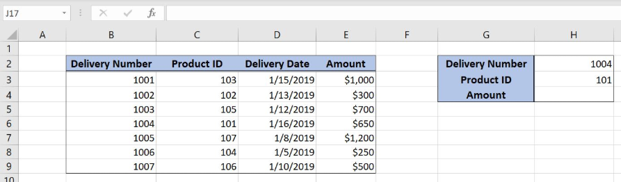 Figure 2. Data that we will use in the example
Performing an INDEX and MATCH with Two Criteria
We want to get an amount, from the lookup table B3:E9, where the Delivery number is 1004 and the Product ID is 101.
The formula looks like:
{=INDEX(E3:E9, MATCH(1, (H2=B3:B9) * (H3=C3:C9), 0))}
The lookup_value parameter of the MATCH function is 1. The lookup_array is (H2=B3:B9) * (H3=C3:C9). The cells H2 and H3 are compared to the arrays and as a result arrays with 0 and 1 is returned. The match_type is 0, which means the approximate match. The result of the MATCH function is the row_num parameter of the INDEX function. The array is the range E3:E9.
To apply the formula, we need to follow these steps:
- Select cell H5 and click on it
- Insert the formula:
=INDEX(E3:E9,MATCH(1,(H2=B3:B9)*(H3=C3:C9),0)) - Press ctrl, shift and enter simultaneously to convert the formula in the array function.
When we evaluate all three comparations in the MATCH function, the lookup_array looks like in Figure 3.
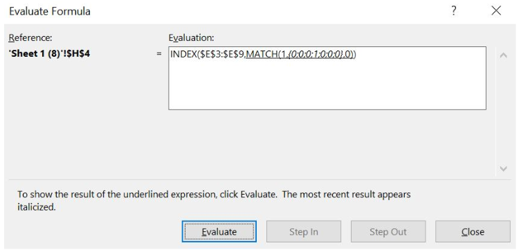 Figure 3. Evaluate the formula
Therefore, the MATCH function returns 4.
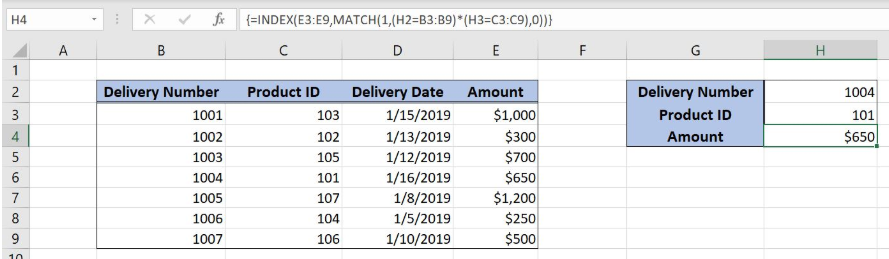 Figure 4. Using the INDEX and MATCH Formula
The 4th row is the row_num parameter of the INDEX function. Finally, the amount from the third row of the lookup_table is the result of the function. The result in the cell H4 is $650.
Most of the time, the problem you will need to solve will be more complex than a simple application of a formula or function. If you want to save hours of research and frustration, try our live Excelchat service! Our Excel Experts are available 24/7 to answer any Excel question you may have. We guarantee a connection within 30 seconds and a customized solution within 20 minutes.


Leave a Comment