

We can use an array formula that is based on the INDEX and MATCH functions to lookup a value based on multiple criteria. The steps below will walk through the process.
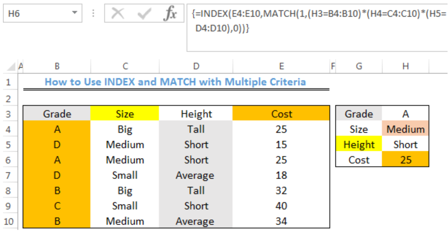 Figure 1- How to Use INDEX and MATCH with Multiple Criteria
General Formula
=INDEX(range1,MATCH(1,(A1=range2)*(B1=range3)*(C1=range4),0))
Formula
=INDEX(E4:E10,MATCH(1,(H3=B4:B10)*(H4=C4:C10)*(H5=D4:D10),0))
Setting up the Data
We will use the INDEX and MATCH functions to get the Cost of the A grade item that is of medium size and short height in figure 2.
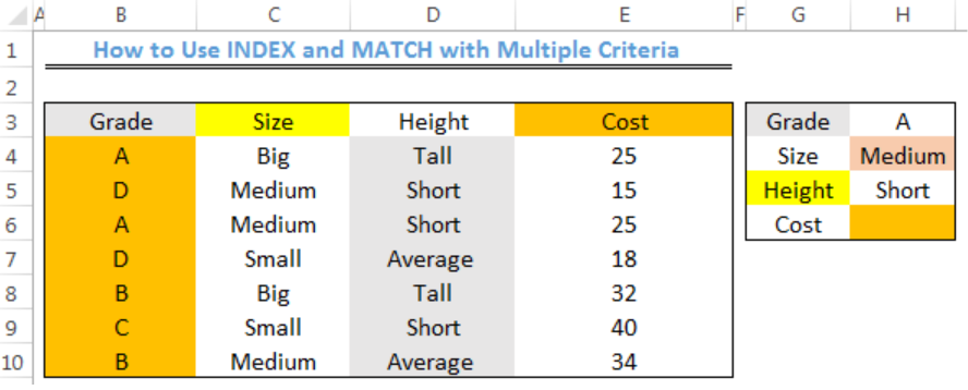 Figure 2 – Setting up the Data
Lookup Cost with INDEX and MATCH with Multiple Criteria
- We will click on Cell H6
- We will insert the formula below into Cell H6
=INDEX(E4:E10,MATCH(1,(H3=B4:B10)*(H4=C4:C10)*(H5=D4:D10),0)) - Because this is an array formula, we will press CTRL+SHIFT+ENTER
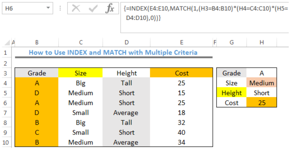 Figure 3- Result for Lookup of Cost with INDEX and MATCH functions with Multiple Criteria
Explanation
In this formula, the MATCH function looks through a one-column range and provides a match based on a specified criteria. Values must be concatenated in a helper column as seen in Column G and Column H. Without this, we can’t supply more than one criteria.
An array of 1 and 0 is used to show the rows that match all three criteria (A, MEDIUM, SHORT). The MATCH FUNCTION is then used to match the first criteria that is found.
From this section of the formula below, we can get the temporary array of 1’s and 0’s:
(H3=B4:B10)*(H4=C4:C10)*(H5=D4:D10)
First, a comparison is made between Cell H3 against all grades, Cell H4 against all Sizes, and Cell H5 against all Height.
An array of TRUE and FALSE is produced. The multiplication operator transforms this into 1s and 0s like this:
{1;0;1;0;0;0;0}*{0;1;1;0;0;0;1}*{0;1;1;0;0;1;0}
The final result is returned to MATCH and MATCH returns 3.
=INDEX(E4:E10,3)
INDEX returns the result as 25.
Instant Connection to an Expert through our Excelchat Service
Most of the time, the problem you will need to solve will be more complex than a simple application of a formula or function. If you want to save hours of research and frustration, try our live Excelchat service! Our Excel Experts are available 24/7 to answer any Excel question you may have. We guarantee a connection within 30 seconds and a customized solution within 20 minutes.


Leave a Comment