

There are several lookup functions in Excel, but not all of them will allow you to use multiple criteria. Here is how you can use the INDEX and MATCH functions to lookup values in Excel with more than one criteria.
How to use INDEX and MATCH with multiple criteria
An array formula can be used to lookup values that meet multiple criteria based on INDEX and MATCH
Formula using INDEX and MATCH
Generic formula syntax to lookup values with INDEX and MATCH with multiple criteria is:
=INDEX(range1, MATCH(1, (criteria1=range2)*(criteria2=range3)*(criteria3=range4), 0))
Where,
- Range1 is the range of cells to lookup for values that meet multiple criteria
- Criteria1,2,3 are cell references to test multiple criteria
- Range2,3,4 are ranges on which each criterion is tested on.
Explanation of formula
Generally, INDEX and MATCH formula has a MATCH set configured in it. This MATCH set helps to look through a one-column range and provides a match that is based on the supplied criteria. For you to supply more than one criteria, you need to use the method of concatenation in a helper column.
This formula uses Boolean logic to create an array of ones and zeros. These are used to represent all rows that match all the three criteria. Then you use the MATCH function to match the first 1 found.
Example
In this example, we want to use the INDEX and MATCH formula to find values in the price column. We shall supply the INDEX and MATCH formula so that it can look through the price column and match a certain cell with the supplied criteria. In this case, we want to look up for a value of shirt, whose size is small, and red in color, then find its price.
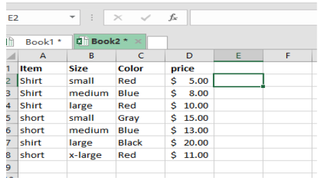
Figure 1: Use INDEX and MATCH to find values
Note that the formula uses Boolean logic to produce an array of ones and zeros to represent all the rows that match the criteria supplied. As we have already mentioned, you need to use an array formula to lookup values with the INDEX and MATCH formula.
In our example above, we put the formula in cell G5 which will be as follows:
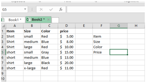
Figure 2: Using INDEX and MATCH with multiple criteria
=INDEX($D$2:$D$8, MATCH(1, (G2=$A$2:$A$8)*(G3=$B$2:$B$8)*(G4=$C$2:$C$8),0))
The answer will be as shown in the figure below:
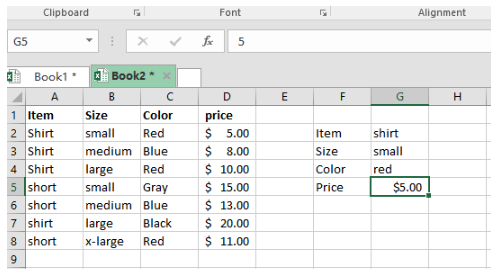
Figure 3 Use INDEX and MATCH to find values
In our working above, the initial results will only consist of {TRUE;FALSE}. But with the use of the multiplication, this is transformed into 0s and 1s.
Non-array version
There is a non-array version of above formula using INDEX and MATCH with multiple criteria. Simply, you need to add another INDEX function to the formula with zero row and one column. This second INDEX function handles the array natively, generated by boolean logic. It returns again the same array to MATCH function because zero trick forces second INDEX to return column 1 from the array as given below.
=INDEX($D$2:$D$8,MATCH(1,INDEX((G2=$A$2:$A$8)*(G3=$B$2:$B$8)*(G4=$C$2:$C$8),0,1),0))
Still need some help with Excel formatting or have other questions about Excel? Connect with a live Excel expert here for some 1 on 1 help. Your first session is always free.


Leave a Comment