

Excel allows a user to get a value from a table using the horizontal lookup. This is possible using the HLOOKUP function, which allows us to get a value from a table organized into rows. This step by step tutorial will assist all levels of Excel users in doing a horizontal lookup.
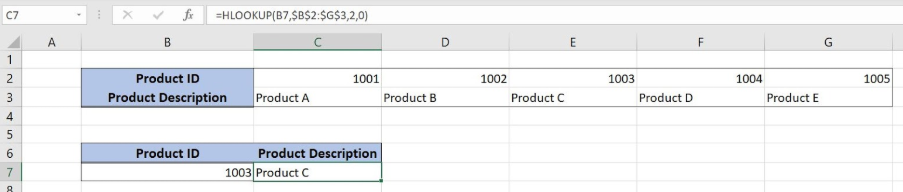 Figure 1. The result of the HLOOKUP function
Syntax of the HLOOKUP Formula
The generic formula for the HLOOKUP function is:
=HLOOKUP(lookup_value, table_array, row_index_num, range_lookup)
The parameters of the HLOOKUP function are:
- lookup_value – a value that we want to find in a table_array
- table_array – a range in which we want to lookup
- row_index_num – a row number in table_array from which we would like to get a value
- range_lookup – default value 0. This means that we want to find an exact match for a lookup value.
Setting up Our Data for the HLOOKUP Function
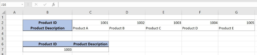 Figure 2. Data that we will use in the HLOOKUP example
In this example, our data is organized horizontally, so we will use the HLOOKUP function. In the range B2:G3, we have a lookup table, while in the cell C7 we want to get a value. Tables consist of the rows “Product ID” and “Product Description”.
Get the Product Description Using the HLOOKUP Function
Our goal is to obtain data from the “Product Description” row in the second table and populate it into the cell C7.
The formula looks like:
=HLOOKUP(B7, $B$2:$G$3, 2, 0)
In our example, the lookup_value is the B3 cell in “Product ID” column. The parameter table_array is $B$2:$G$3 because we want to find value from the range B2:G3. Row_index_num has value 2, as we want to pull value from the second row of the range. Finally, range_lookup has value 0, because we want to find an exact match of “Product ID” values.
To apply the HLOOKUP function, we need to follow these steps:
- Select cell C7 and click on it
- Insert the formula:
=HLOOKUP(B7,$B$2:$G$3,2,0) - Press enter
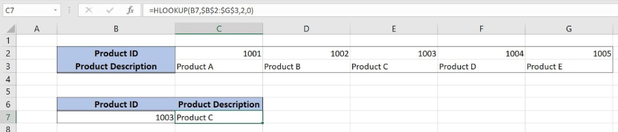 Figure 3. Get the product description using the HLOOKUP function
As a result, we will get Product C in the cell C7. As you can see, the value of “Product Description” in E3 in the 1st table is Product C. The function pulls this value and returns it to the cell C7 as a result.
Most of the time, the problem you will need to solve will be more complex than a simple application of a formula or function. If you want to save hours of research and frustration, try our live Excelchat service! Our Excel Experts are available 24/7 to answer any Excel question you may have. We guarantee a connection within 30 seconds and a customized solution within 20 minutes.


Leave a Comment