

We can find the First Non-Blank Value (text or number) in a list by applying the INDEX, MATCH and ISBLANK functions. We will also use the ISTEXT function instead of the ISBLANK function to find the First Text Value in our list. We will follow the simple steps below to achieve our objective.
![]() Figure 1: Results for First Non-blank Value and Text Value in a List
Figure 1: Results for First Non-blank Value and Text Value in a List
Setting up the Data
- We will set up our data by inputting the numeric and text values into Column A, titled, LIST.
- We will type FIRST NON-BLANK VALUE and FIRST TEXT VALUE into Cell B5 and Cell C5 respectively. Refer to figure 1.
How to get the First Non-blank Value in a List
Syntax:
=INDEX(range,MATCH(FALSE,ISBLANK(range),0))
For us to get the first non-blank value in our list, we will do the following:
- We will click on Cell B6
- We will type or copy and paste the formula below into the cell
=INDEX(A4:A11,MATCH(FALSE,ISBLANK(A4:A11),0))
![]() Figure 2: How to Find the First Non-blank Value in a List
Figure 2: How to Find the First Non-blank Value in a List
Once we have inputted the formula, we will press CTRL + SHIFT + ENTER. We will have the result as shown in figure 3.
![]() Figure 3: Result for the First Non-blank Value in a List
Figure 3: Result for the First Non-blank Value in a List
Explanation of the formula
ISBLANK(A4:A11)
The ISBLANK function tests the cells in the range A4:A11 if there are blank cells or not. It then returns an array that looks like this:
{TRUE;TRUE;FALSE;FALSE;FALSE;FALSE;TRUE;FALSE}
TRUE means that a cell is blank. FALSE means that a cell is not blank.
MATCH(FALSE,ISBLANK(A4:A11),0)
MATCH function finds the first FALSE value in the above array (A4:A11) and returns the CELL POSITION of that FALSE value in the array. In this case, the Cell Position in the array is Cell A6.
INDEX(A4:A11,MATCH(…))
Once the first non-blank cell is found, INDEX function returns its value AS TRUE WHETHER IT IS A TEXT OR NUMERIC VALUE.
How to get the First Text Value in a List
Syntax:
=INDEX(range,MATCH(TRUE,ISTEXT(range),0))
For us to get the first text value in our list, we will do the following:
- We will click on Cell C6
- We will type or copy and paste the formula below into the cell
=INDEX(A4:A11,MATCH(TRUE,ISTEXT(A4:A11),0))
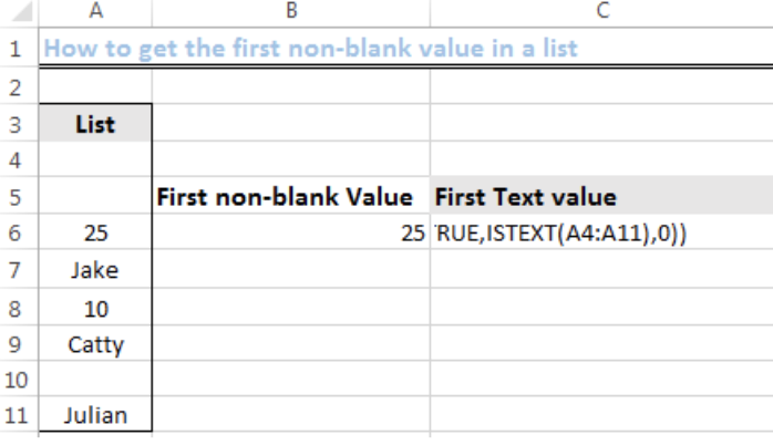 Figure 4: How to Find the First Text Value in a List
Once we have inputted the formula, we will press CTRL + SHIFT + ENTER. We will have the result as shown in figure 5.
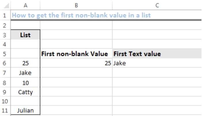 Figure 5: Result for the First Text Value in a List
Explanation of the formula
ISTEXT(A4:A11)
The ISTEXT function tests the cells in the range A4:A11 if there are cells that contain text or not. It then returns an array that looks like this:
{FALSE; FALSE;FALSE;TRUE;FALSE; TRUE;FALSE;TRUE}
TRUE means that a cell CONTAINS A TEXT VALUE. FALSE means that a cell doesn’t contain a text value.
MATCH(TRUE,ISTEXT(A4:A11),0)
MATCH function finds the first TRUE value in the above array (A4:A11) and returns the CELL POSITION of that TRUE value in the array. In this case, the Cell Position in the array is Cell A7.
INDEX(A4:A11,MATCH(…))
Once the first TEXT-CONTAINING CELL is found, INDEX function returns its value AS TRUE.
Instant Connection to an Expert through our Excelchat Service:
Most of the time, the problem you will need to solve will be more complex than a simple application of a formula or function. If you want to save hours of research and frustration, try our live Excelchat service! Our Excel Experts are available 24/7 to answer any Excel question you may have. We guarantee a connection within 30 seconds and a customized solution within 20 minutes.


Leave a Comment