

If you want to search for a word or a string in an Excel sheet, a check can be made on each cell to look for that string or word. Moreover, a counter can also be initialized that will intimate the number of repetitions of a string in a selected number of cells.
Extract partial matches in Excel
Extraction of all the matches can be made by using array formula based on partial match using AGGREGATE and INDEX functions, with SEARCH and ISNUMBER functions to act as supporting functions. The generic formula for this purpose is written below.
Formula
=IF(F4>count,"",INDEX(data,AGGREGATE(15,6,(ROW(data)-ROW($B$4)+1)/ISNUMBER(SEARCH(value,data)),F4)))
Explanation of formula
Above written general formula uses IF, INDEX, AGGREGATE, ROW, ISNUMBER and SEARCH functions in it. The detailed description of these functions is presented below.
Working of Extract All Partial Matches’ Formula
The major role played in this formula is that of the INDEX function, in support of AGGREGATE used to find the “nth match” for each and every row in the selected area. The general form of INDEX function is written below:
=INDEX(data,nth match_formula)
The working principle to extract all the partial matches lies in figuring out that which row in the data matches the search string and reporting about the position of each matched value to this INDEX function. This can be performed with the assistance of AGGREGATE function which must be configured as follows:
=AGGREGATE(15,6,(ROW(data)-ROW($B$4)+1)/ISNUMBER(SEARCH(value,data)),F4)
The first parameter in the AGGREGATE function sets it to act as the SMALL function and return the nth smallest value. The second parameter, 6, implies the SMALL function to ignore the errors. The 3rd argument returns an array of matching results. The 4th argument consists of Xn i.e. the cell number to define the nth value.
The AGGREGATE operation requires an array to be passed to it as an input parameter. Following formula is used to create an array to be passed as the 3rd argument inside the AGGREGATE function.
(ROW(data)-ROW($B$4)+1)/ISNUMBER(SEARCH(value,data))
The ROW function is used here to return the relatively low numbers. Moreover, SEARCH and ISNUMBER are used to compare the string against the values entered in the data array, which generates a boolean array consisting of TRUE / FALSE entries, which mean 1 and 0 respectively.
The result is that the row numbers in which the search text is found, are divided by unity and are retained. While the row numbers of non-matching values are divided by 0 and are turned into #DIV/0 errors. As the AGGREGATE function is set to 6, i.e. to ignore error’ option. It ignores the errors and returns the smallest number in residual values, using the value in the F column for nth.
Counting the Search Results
For counting the number of results retrieved with the help of the above formula, is counted by using the formula written below.
=COUNTIF(data,"*"&search&"*")
This check on the count cell prevents the AGGREGATE and INDEX functions from running once. When all the matching values, with that of the search string, have been retrieved.
Example
A list of some American states has been considered, which can be checked for the states having the text “new” at the starting place of their name. The following figure shows the Excel sheer that is to be considered for this example.
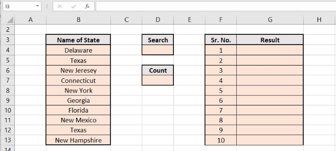 Figure 1. Sample sheet for extracting all partial matches from the data
To get the value of count corresponding to the search criteria, enter the following formula in cell “D7”
=COUNTIF(data,"*"&search&"*")
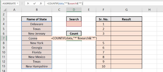 Figure 2. Getting the count value for the matched results from the data
Now as explained earlier enter the formula for extacting all partial matches to the cell G4 and copy this formula to all the cells below it:
=IF(F4>count,"",INDEX(data,AGGREGATE(15,6,(ROW(data)-ROW($B$4)+1)/ISNUMBER(SEARCH(search,data)),F4)))
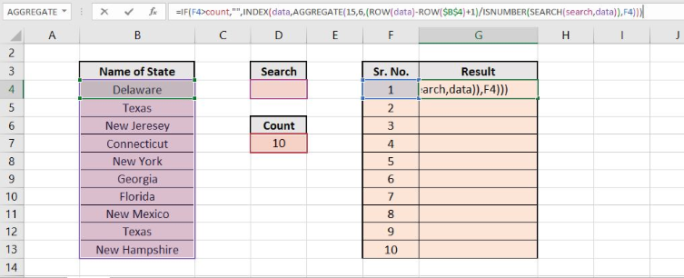 Figure 3. Entering the formula to extract all partial matches from data
As the search criteria have not been defined yet, that’s why the count is showing 10 i.e. the total number of entries in the data. Now for checking, type any word or a string in the cell below the search tab, you will get the corresponding entries which will contain the matches in the result section.
For example, the results for typing “new” in the search section gives the following result:
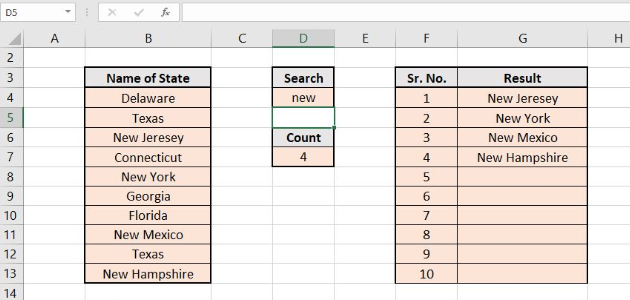 Figure 4. Results of partial matches for “new” from data
Similarly, for search criteria “co” results are presented below:
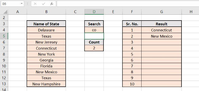 Figure 5. Results of partial matches for “co” from data
Still need some help with Excel formatting or have other questions about Excel? Connect with a live Excel expert here for some 1 on 1 help. Your first session is always free.


Leave a Comment